2.0.2: DEA Mangrove Canopy Cover (Landsat)

Mangrove Canopy Cover 25m 2.0.2

Version:: 2.0.2 (See latest version)
Product types:: Derivative, Raster
Update frequency:: Deprecated

Old version

This is an old version of the product. See the latest version.

Overview

About

Tracking changes in the extent and canopy density of mangroves, Digital Earth Australia (DEA) Mangrove Canopy Cover reveals how these extraordinary trees may be responding to sea level rise, severe tropical cyclones, drought, climatic cycles, changing temperatures and large storm events.

Key details

Collection	Geoscience Australia Landsat Collection 2
Persistent ID	135270
Licence	Creative Commons Attribution 4.0 International Licence

Publications

Lymburner, L., Bunting, P., Lucas, R., Scarth, P., Alam, I., Phillips, C., Ticehurst, C., & Held, A. (2020). Mapping the multi-decadal mangrove dynamics of the Australian coastline. Remote Sensing of Environment, 238, 111185. https://doi.org/10.1016/j.rse.2019.05.004

Details

Background

Mangroves provide a diverse array of ecosystem services but these are impacted upon by both natural and anthropogenic drivers of change. In Australia, mangroves are protected by law and hence the natural drivers predominate.

It is important to know the extent and canopy density of mangroves in Australia so that we can measure how mangroves are responding to sea level rise, severe tropical cyclones and climatic cycles.

What this product offers

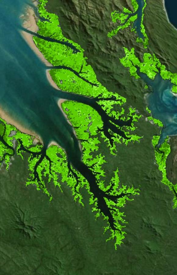
This product provides valuable information about the extent and canopy density of mangroves for each year between 1987 and 2018 for the entire Australian coastline.

The canopy cover classes are:

20–50%	Pale green
50–80%	Mid green
80–100%	Dark green

The product consists of a sequence (one per year) of 25 m resolution maps that are generated by analysing the Landsat fractional cover developed by the Joint Remote Sensing Research Program and the Global Mangrove Watch layers developed by the Japanese Aerospace Exploration Agency.

Applications

The sequence of mangrove maps makes it possible to see how the extent of mangroves is changing over time. The maps can be used to understand how mangroves respond to disturbance events such as severe tropical cyclones. The maps can also be used to improve our representation of the ecosystem services provided by mangroves, which include:

Coastal protection
Carbon storage
Providing nursery grounds for commercially important fish and prawn species
Providing habitat for migratory and endemic bird species

Technical information

To determine annual national level changes in mangroves between 1987 and 2016, their extent (by canopy cover type) and dynamics were quantified using dense time-series (nominally every 16 days cloud permitting) of 25 m spatial resolution Landsat sensor data available within Digital Earth Australia (DEA).

The potential area that mangroves occupied over this period was established as the union of mangrove maps generated for 1996, 2007-2010 and 2015/16 through the Japanese Aerospace Exploration Agency (JAXA) Global Mangrove Watch (GMW), and then refined using tasseled cap wetness dynamics and State and Territory mangrove mapping products. Within this area the 10th percentile of the green vegetation fraction of the FC-PERCENTILE_25_2.0.0 (GVpc10) was retrieved. The percentage Planimetric Canopy Cover (PCC%) for each Landsat pixel was estimated using a relationship between GVpc10 and LiDAR-derived PCC% (< 1 m resolution and based on LIDAR acquisitions from all states supporting mangroves, excluding Victoria).

The resulting annual maps of mangrove extent and cover indicate that the total area of mangrove forest (canopy cover > 20%; resolvable at the Landsat resolution) varied from a minima of 10,062 km2 in 1992 to a maxima of 10,642 km2 in 2010, declining to 10,434 km2 in 2016. In 2010 (maximum extent), the forests were classified as closed canopy (38.8%), open canopy (49.0%) and woodland mangrove (12.2%). The majority of change occurred along the northern Australian coastline and was concentrated in the major gulfs and sounds.

Lineage

The product development methodology is outlined in the following steps:

Calculate the green fractional cover (GVpc) from all available cloud-free Landsat pixels for each year of observation and compare these over an annual time series to identify areas where green cover persists throughout the year.
Establish a relationship between the 10th percentile of green fraction (GVpc10) observed within a year and Planimetric Canopy Cover percentage (PCC%) derived from < 1 m spatial resolution canopy masks derived from LIght Detection And Ranging (LiDAR) with this representing a unit that relates directly to forest cover.
Constrain the PCC% estimates to areas known to contain mangroves, with reference to the Japanese Aerospace Exploration Agency’s (JAXA) Kyoto and Carbon (K&C) Initiative Global Mangrove Watch (GMW) thematic layers for 1996, 2007-10 and 2015/16 with additional areas identified using tasseled cap wetness and State and Territory mangrove mapping products.
Apply PCC% thresholds to map mangrove forest extent (based on a pre-determined 20 PCC% threshold) and differentiate structural categories, namely, woodland (20-50 %), open forest (50-80 %), and closed forest (> 80 %).
Quantify the change in the extent of mangrove forest and canopy cover types over the period 1987 to 2018 at a national scale and establish relevance at regional (e.g., State/Territory) and local levels.

Processing steps

Fractional Cover Processing

References

Quality

Accuracy

There is a strong \(r2 = 0.99\) correlation between predicted and observed canopy cover based on an independent set of LiDAR surveys. It is worth noting however that the per pixel RMSE is high (26%) because the per pixel canopy cover estimates from the LiDAR are very sensitive to the location of the 25 meter grid placement. The accuracy of the green fraction cover percentage estimates is inherited from the FC product. Based on the comparison with 1565 independent field data points the green cover product has an overall Root Mean Squared Error (RMSE) of 11.9%.

The Global Mangrove Watch polygon that was created using the methods described in Lucas et al. 2014 doi:10.1071/MF13177 was used to provide a consistent reference frame. However this product has limitations that will impact on the Mangrove_25 product. Areas that were mangrove prior to 2010 but were not identified as mangrove in 2010 may be omitted from this sequence of maps. Likewise some small areas of coastal non-mangrove woody vegetation (Casuarina and Melaleuca) are included in the GMW mangrove extent polygons. Whilst all reasonable efforts have been taken to minimise this, some errors of commission (non mangrove being identified as mangrove) will still occur.

For more information, see Lymburner et al. (2020).

Quality assurance

The quality of this product is related to both the quality of the Fractional_Cover_25 product and the PQ_25 product. During periods when only one satellite is operating (1987 to 2003, and 2011/12) the 10th percentile will sometimes contain cloud/cloud shadow artefacts due to the low number of observations per year in these years. This is typically problematic in cloud prone areas such as the Wet Tropics. This can be mitigated in two ways, either by excluding these years from analysis, or by using the PQ_COUNT layers to identify locations that had a low number of observations in a given year.

History

Other versions

You can find the history in the latest version of the product.

Credits

Acknowledgments

Landsat data is provided by the United States Geological Survey (USGS) through direct reception of the data at Geoscience Australias satellite reception facility or download.

The fractional cover algorithm was developed by the Joint Remote Sensing Research Program (JRSRP) and is described in Scarth et al. (2010). While originally calibrated in Queensland, a large collaborative effort between The Department of Agriculture and ABARES and State and Territory governments to collect additional calibration data has enabled the calibration to extend to the entire Australian continent. FC_25 was made possible by new scientific and technical capabilities, the collaborative framework established by the Terrestrial Ecosystem Research Network (TERN) through the National Collaborative Research Infrastructure Strategy (NCRIS), and collaborative effort between state and Commonwealth governments.

This product is the result of a collaboration between Geoscience Australia, the University of Aberyswyth, CSIRO, the Joint Remote Sensing Research Program and the Terrestrial Ecosystem Research Network

License and copyright

Released under Creative Commons Attribution 4.0 International Licence.