DEA Intertidal Extents (Landsat)

Intertidal Extents Model 25m

Version:: 2.0.0 (Latest)
Product types:: Derivative, Raster
Time span:: 1986 – 2016
Update frequency:: As needed
Next update:: No updates planned
Product ID:: item_v2

Overview

About

Understanding the boundaries of the ‘intertidal zone’ — the strip of coastal land revealed and concealed daily by ocean tides — has long been a challenge. Digital Earth Australia (DEA) Intertidal Extents gives definition to complex and ephemeral landscapes.

The dataset provides information on the lowest (LOT) and highest (HOT) observed tides for a chosen geographic cell, revealing the satellite-observed tidal range (HOT-LOT) for any given location.

New version in development

A new version of this product is being developed as part of the DEA Intertidal product suite. Subscribe to the DEA newsletter to be notified of product releases.

Access the data

For help accessing the data, see the Access tab.

Data explorer

Explore data availability

Access the data on NCI

Get the data online

Web Map Service (WMS)

Get via web service

Key details

Parent product(s)	Landsat 5, 7 and 8 NBAR and Observational Attributes (Collection 2)
Collection	Geoscience Australia Landsat Collection 2
DOI	10.4225/25/5a602cc9eb358
Licence	Creative Commons Attribution 4.0 International Licence

Cite this product

Data citation

Sagar, S., Roberts, D., Bala, B., Lymburner, L., 2017. Intertidal Extents Model 25m v. 2.0.0. Geoscience Australia, Canberra. http://dx.doi.org/10.4225/25/5a602cc9eb358

Paper citation

Sagar, S., Roberts, D., Bala, B., Lymburner, L., 2017. Extracting the intertidal extent and topography of the Australian coastline from a 28 year time series of Landsat observations. Remote Sensing of Environment 195, 153-169. https://doi.org/10.1016/j.rse.2017.04.009

Publications

Sagar, S., Roberts, D., Bala, B., & Lymburner, L. (2017). Extracting the intertidal extent and topography of the Australian coastline from a 28 year time series of Landsat observations. Remote Sensing of Environment, 195, 153–169. https://doi.org/10.1016/j.rse.2017.04.009

Details

Background

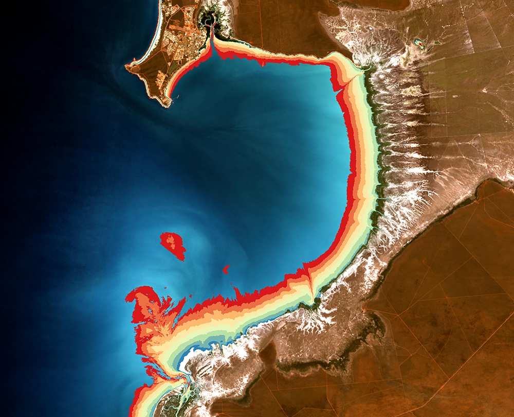
Intertidal zones are those which are exposed to the air at low tide and underwater at high tide. These include sandy beaches, tidal flats, rocky shores and reefs.

Intertidal zones form critical habitats for a wide range of organisms, but are faced with increasing threats, including coastal erosion and a rise in sea levels.

Accurate knowledge of the extent and topography of these regions can help assess where these threats will have the greatest impact, and provide essential information to underpin monitoring and management strategies. This data is challenging to acquire using traditional survey methods given the dynamic nature of intertidal zones and length of the Australian coastline.

What this product offers

This product is a national dataset of the exposed intertidal zone: the land between the observed highest and lowest tide. It provides the extent and topography of the intertidal zone of Australia’s coastline (excluding off-shore Territories).

This information was collated using observations in the Landsat archive since 1986. This product can be a valuable complementary dataset to both onshore LiDAR survey data and coarser offshore bathymetry data, enabling a more realistic representation of the land and ocean interface.

Applications

Understanding the extent and topography of the Australian intertidal zone
Environmental monitoring of migratory bird species
Habitat mapping in coastal regions
Hydrodynamic modelling
Geomorphology studies of features in the intertidal zone

Technical information

The Intertidal Extents Model product is a national scale gridded dataset characterising the spatial extents of the exposed intertidal zone, at intervals of the observed tidal range (Sagar et al. 2017). The current version (2.0) utilises all Landsat observations (5, 7, and 8) for Australian coastal regions (excluding off-shore Territories) between 1986 and 2016 (inclusive).

Datasets

The Intertidal Extents Model (ITEM v2.0) consists of three datasets derived from the Landsat NBAR data managed in Digital Earth Australia for the period 1986 to 2016

Dataset 1: ITEM v2.0 TIDAL MODEL

The ITEMv2_tidalmodel.shp identifies the location and extents of the 306 polygons (Figure 1) used in the product, defined by the Continental Scale tidal modelling framework (see Processing Step: Create a continental scale tidal modelling framework). The shapefile also includes information on the lowest (LOT) and highest (HOT) observed tides for the cell, and hence the observed tidal range (HOT-LOT), based on tidal modelling for the time of acquisition of each of the corresponding Landsat observations in the cell polygon.

Attributes:


ID	Unique Polygon Identifier
lon	Polygon Centroid Longitude
lat	Polygon Centroid Latitude
LOT	Lowest Observed Tide – The lowest modelled tidal height based on the acquisition times of all observations in the polygon. Relative to Mean Sea Level (MSL) (m).
HOT	Highest Observed Tide – The highest modelled tidal height based on the acquisition times of all observations in the polygon. Relative to Mean Sea Level (MSL) (m).
LMT	Lowest Modelled Tide - The lowest modelled tidal height based on the OTPS model for the full period of the archive. Relative to Mean Sea Level (MSL) (m).
HMT	Highest Modelled Tide - The highest modelled tidal height based on the OTPS model for the full period of the archive. Relative to Mean Sea Level (MSL) (m).

ITEM v2 polygon extents — Figure 1: Polygon extents for ITEM v2.

Dataset 2: THE RELATIVE EXTENTS MODEL v2.0

The Relative Extents Model (item_v2) utilises the tidal information attributed to each Landsat observation to indicate the spatial extent of intertidal substratum exposed at percentile intervals of the observed tidal range for the cell. The dataset consists of 306 raster files (NETCDF and Geotiff) corresponding to polygons of the continental scale tidal model.

Naming convention:

ITEM_REL_PolygonID_CentroidLongitude_CentroidLatitude

E.g. ITEM_REL_95_153.67_-28.77.tif

Single Band Integer Raster:


0	Always water
1	Exposed at lowest 0-10% of the observed tidal range
2	Exposed at 10-20% of the observed tidal range
3	Exposed at 20-30% of the observed tidal range
4	Exposed at 30-40% of the observed tidal range
5	Exposed at 40-50% of the observed tidal range
6	Exposed at 50-60% of the observed tidal range
7	Exposed at 60-70% of the observed tidal range
8	Exposed at 70-80% of the observed tidal range
9	Exposed at highest 80-100% of the observed tidal range (land)
-6666	No Data

Dataset 3: THE CONFIDENCE LAYER v2.0

The Confidence Layer (item_v2_conf) reflects the confidence level of the Relative Extents Model, based on the distribution of classification metrics (see Processing Step: Calculate NDWI for each Observation) within each of the percentile intervals of the tidal range. The layer should be used to filter region/pixels in the model where the derived spatial extents may be adversely affected by data and modelling errors. The dataset consists of 306 raster files (NETCDF and Geotiff) corresponding to polygons of the continental scale tidal model.

Naming Convention:

ITEM_STD_PolygonID_CentroidLongitude_CentroidLatitude

E.g. ITEM_STD_95_153.67_-28.77.tif

Single Band Integer Raster:


-6666	No Data – Model is invalid. Indicates pixels where data quality and/or number of observations have resulted in no available observations in one or more of the percentile interval subsets.
All other values	The pixel-based average of the NDWI standard deviations calculated independently for each percentile interval of the observed tidal range.

Lineage

The Intertidal Extents Model product analyses GA’s historic archive of satellite imagery to derive a model of the spatial extents of the intertidal zone throughout the tidal cycle. The model can assist in understanding the relative elevation profile of the intertidal zone, delineating exposed areas at differing tidal heights and stages.

The product differs from previous methods used to map the intertidal zone which have been predominately focused on analysing a small number of individual satellite images per location (e.g Ryu et al., 2002; Murray et al., 2012). By utilising a full 30 year time series of observations, the methodology enables us to overcome the requirement for clear, high quality observations acquired concurrent to the time of high and low tide.

Processing steps

1. Create a continental scale tidal modelling framework

Create a continental scale tidal modelling framework utilising continental scale tidal prediction software developed by Oregon State University (OTPS, Egbert and Erofeeva, 2002, 2010). OTPS tide heights were attributed to Landsat observations in the DEA at corresponding times and dates, per location

The modelling process utilises continental scale tidal prediction software developed by Oregon State University (OTPS, Egbert and Erofeeva, 2002, 2010). OTPS tide heights were attributed to Landsat observations in the DEA at corresponding times and dates, per location.

To account for geographic and seasonal variations in tidal regimes and ranges, twelve tidal height rasters of the study region at 1km resolution were created utilising the OTPS model, at a randomly selected monthly epoch across a full year. Utilising these raster layers, the tidal modelling spatial framework was constructed with the following steps:

Perform a multi-resolution segmentation using eCognition software, utilising all twelve tidal height inputs, to create a spatial representation of the multi-epoch tidal variation across the continent.
Extract the centroids of the object segments created in eCognition and generate a Voronoi Polygon tessellation of the region.
Perform a visual assessment and manual adjustment of the Voronoi polygon boundaries and nodes to ensure alignment with natural boundaries and coastal/island features.

Through this process, the coastal zone is divided into Voronoi polygons that capture the tidal complexity of the Australian coast, with areas of complex tidal behaviour represented using smaller polygons. The nodes of the polygons can then be used for the tidal attribution process as described in Sagar et al., (2017).

2. Apply the Oregon State University tidal model to coastline cells/polygons

The Oregon State University Tidal Prediction Software (OTPS) TPX08 Atlas Model is applied to each coastal cell, to model tidal heights (MSL) at the nominated cell centroid or node location.

3. Attribute coastal cells with a tidal height

All observations within the nominated cell/polygon and time period is attributed with a tidal height, relative to Mean Sea Level (MSL), corresponding to the time of observation acquisition and derived cell/polygon centroid or node.

4. Sort time series of observations based on tidal height

The time-series of observations for each cell/polygon is then sorted based on the modeled tidal height, and split into subsets representing percentile intervals of the observed tidal range (OTR) for that cell/polygon.

5. Mask tile observations for pixel quality

Each tile observation is masked for pixel quality based on the DEA PQA layer to exclude pixels flagged for cloud, band saturation and contiguity.

6. Calculate NDWI for each observation

The Normalised Difference Water Index (NDWI) (McFeeters, 1996) is calculated for each observation, and a pixel based median NDWI composite derived for each percentile interval of the cell’s OTR. The pixel-based standard deviation of NDWI values within each percentile interval is also recorded for use in the Confidence Layer.

7. Create binary NDWI layers and combine to create Relative Extents Model

Binary Land/Water layers are created from the NDWI composites for each tidal interval using a standard threshold. These are then combined to create the Relative Extents Model. For full methodology and process details see Sagar et al. 2017.

References

Egbert, G.D., Erofeeva, S.Y., 2010. The OSU TOPEX/Poseiden Global Inverse Solution TPXO [WWW Document]. TPXO8-Atlas Version 10. URL http://volkov.oce.orst.edu/tides/global.html (accessed 2.15.16).

Egbert, G.D., Erofeeva, S.Y., 2002. Efficient Inverse Modeling of Barotropic Ocean Tides. J. Atmospheric Ocean. Technol. 19, 183–204. https://doi.org/10.1175/1520-0426(2002)019%3C0183:EIMOBO%3E2.0.CO;2

Sagar, S., Phillips, C., Bala, B., Roberts, D., & Lymburner, L. (2018). Generating continental scale pixel-based surface reflectance composites in coastal regions with the use of a multi-resolution tidal model. Remote Sensing, 10(3), 480. https://doi.org/10.3390/rs10030480

Quality

Accuracy

Due the sun-synchronous nature of the various Landsat sensor observations; it is unlikely that the full physical extents of the tidal range in any cell will be observed. Hence, terminology has been adopted for the product to reflect the highest modelled tide observed in a given cell (HOT) and the lowest modelled tide observed (LOT) (Figure 1). These measures are relative to Mean Sea Level, and have no consistent relationship to Lowest (LAT) and Highest Astronomical Tide (HAT).

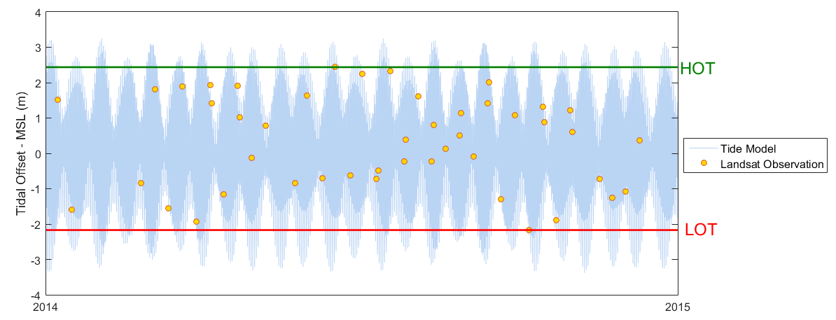
tide range — Figure 1: Tidal range showing the HOT and LOT.

The inclusion of the lowest (LMT) and highest (HMT) modelled tide values for each tidal polygon in the ITEMv2_tidalmodel dataset indicates the highest and lowest tides modelled for that location across the full time series by the OTPS model. The relative difference between the LOT and LMT (and HOT and HMT) heights gives an indication of the extent of the tidal range represented in the Relative Extents Model.

As in ITEM v1.0, v2.0 contains some false positive land detection in open ocean regions. These are a function of the lack of data at the extremes of the observed tidal range, and features like glint and undetected cloud in these data poor regions/intervals. Methods to isolate and remove these features are in development for future versions.

Issues in the DEA archive and data noise in the Esperance, WA region off Cape Le Grande and Cape Arid (Polygons 236, 201, 301) has resulted in significant artefacts in the model, and use of the model in this area is not recommended.

Quality assurance

The Confidence layer is designed to assess the reliability of the Relative Extent Model. Within each tidal range percentile interval, the pixel-based standard deviation of the NDWI values for all observations in the interval subset is calculated. The average standard deviation across all tidal range intervals is then calculated and retained as a quality indicator in this product layer.

The Confidence Layer reflects the pixel based consistency of the NDWI values within each subset of observations, based on the tidal range. Higher standard deviation values indicate water classification changes not based on the tidal cycle, and hence lower confidence in the extent model. Possible drivers of these changes include:

Inadequacies of the tidal model, due perhaps to complex coastal bathymetry or estuarine structures not captured in the model. These effects have been reduced in ITEM v2.0 compared to previous versions, through the use of an improved tidal modelling framework (see Sagar et al. 2018)
Change in the structure and exposure of water/non-water features NOT driven by tidal variation. For example, movement of sand banks in estuaries, construction of man-made features (ports etc.).
Terrestrial/Inland water features not influenced by the tidal cycle.

Access

Access the data

Explore data availability	Data explorer	Learn how to use the DEA Explorer
Get the data online	Access the data on NCI	Learn how to access the data via AWS
Get via web service	Web Map Service (WMS)	Learn how to use DEA’s web services

History

Old versions

No old versions available.

Changelog

ITEM v2.0 has implemented an improved tidal modelling framework (see Sagar et al. 2018 and Processing Step: Create a continental scale tidal modelling framework) over that utilised in ITEM v1.0. The expanded Landsat archive within the Digital Earth Australia (DEA) has also enabled the model extent (Figure 1) to be increased to cover a number of offshore reefs, including the full Great Barrier Reef and southern sections of the Torres Strait Islands.

The DEA archive and new tidal modelling framework has improved the coverage and quality of the ITEM v2.0 relative extents model, particularly in regions where AGDC cell boundaries in ITEM v1.0 produced discontinuities or the imposed v1.0 cell structure resulted in poor quality tidal modelling (see Sagar et al. 2017).

Examples of regions in ITEM v2.0 where these significant improvements have been noted include:

Dampier Peninsula and King Sound, WA. Improved modelling within King Sound has removed the discontinuities seen at cell boundaries in ITEM v1.0, and expanded the extent of intertidal region being mapped.
Tiwi Islands, Coburg Pensinsula and Croker Island, NT. Poor spatial representation of the regions tidal regimes in ITEM v1.0 has been improved in v2.0 resulting in extensive onshore reefs and mudflats now being mapped.
The full Great Barrier Reef has been mapped, detailing reef structures which expose at low tide. Algorithm amendments have reduced the false positive exposed surface detections resulting from glint and sun glitter.
Broad Sound, QLD. Improved tidal modelling has resulted in a smoother intertidal extent map, and a greatly improved confidence layer value for the region.
Improvements in the coverage of the DEA archive has allowed many regions unresolved in ITEM v1.0 and showing as ‘no data’ to be modelled successfully in ITEM 2.0. For example, Mornington Island, QLD, Eastern sections of Fraser Island, QLD and pensinsulas in Bowling Green Bay National Park near Townsville, QLD.

Credits

Acknowledgments

This research was undertaken with the assistance of resources from the National Computational Infrastructure (NCI), which is supported by the Australian Government.

License and copyright

Released under Creative Commons Attribution 4.0 International Licence.