DEA Surface Reflectance OA (Sentinel-2A MSI)
DEA Surface Reflectance OA (Sentinel-2A MSI)
Geoscience Australia Sentinel-2A Observation Attributes Collection 3
- Version:
3.2.1 (Latest)
- Product types:
Baseline, Raster
- Time span:
12/07/2015 – Present
- Update frequency:
Daily
- Product ID:
ga_s2am_ard_3
About
DEA Surface Reflectance OA (Sentinel-2A MSI) is part of a suite of Digital Earth Australia’s (DEA) Surface Reflectance datasets that represent the vast archive of images captured by the US Geological Survey (USGS) Landsat and European Space Agency (ESA) Sentinel-2 satellite programs, which have been validated, calibrated, and adjusted for Australian conditions — ready for easy analysis.
Access the data
For help accessing the data, see the Access tab.
DEA Maps
DEA Explorer
Access the data on AWS
Access the data on NCI
Code examples
Web Services
Key details
Collection |
Geoscience Australia Sentinel-2 Collection 3 |
DOI |
|
Licence |
Cite this product
Data citation |
Geoscience Australia, 2022. Geoscience Australia Sentinel-2A Observation Attributes Collection 3 - DEA Surface Reflectance OA (Sentinel-2A MSI). Geoscience Australia, Canberra. https://dx.doi.org/10.26186/146568
|
Background
Sub-product
This is a sub-product of DEA Surface Reflectance (Sentinel-2A). See the parent product for more information.
The contextual information related to a dataset is just as valuable as the data itself. This information, also known as data provenance or data lineage, includes details such as the data’s origins, derivations, methodology and processes. It allows the data to be replicated and increases the reliability of derivative applications.
Data that is well-labelled and rich in spectral, spatial and temporal attribution can allow users to investigate patterns through space and time. Users are able to gain a deeper understanding of the data environment, which could potentially pave the way for future forecasting and early warning systems.
The surface reflectance data produced by NBART requires accurate and reliable data provenance. Attribution labels, such as the location of cloud and cloud shadow pixels, can be used to mask out these particular features from the surface reflectance analysis, or used as training data for machine learning algorithms. Additionally, the capacity to automatically exclude or include pre-identified pixels could assist with emerging multi-temporal and machine learning analysis techniques.
What this product offers
This product contains a range of pixel-level observation attributes (OA) derived from satellite observation, providing rich data provenance:
null pixels
clear pixels (fmask)
cloud pixels (fmask)
cloud shadow pixels (fmask)
snow pixels (fmask)
water pixels (fmask)
clear pixels (s2cloudless)
cloud pixels (s2cloudless)
cloud probability (s2cloudless)
spectrally contiguous pixels
terrain shaded pixels.
It also features the following pixel-level information pertaining to satellite, solar and sensing geometries:
solar zenith
solar azimuth
satellite view
incident angle
exiting angle
azimuthal incident
azimuthal exiting
relative azimuth
relative slope
timedelta.
Technical information
How observation attributes can be used
This product provides pixel- and acquisition-level information that can be used in a variety of services and applications. This information includes:
data provenance, which:
denotes which inputs/parameters were used in running the algorithm
demonstrates how a particular result was achieved
can be used as evidence for the reasoning behind particular decisions
enables traceability
training data for input into machine learning algorithms, or additional likelihood metrics for image feature content, where pre-classified content includes:
cloud
cloud shadow
snow
water
additional pixel filtering (e.g. exclude pixels with high incident angles)
pre-analysis filtering based on image content (e.g. return acquisitions that have less than 10% cloud coverage)
input into temporal statistical summaries to produce probability estimates on classification likelihood
This product allows you to screen your data for undesired anomalies that can occur during any phase: from the satellite’s acquisition, to the processing of surface reflectance, which relies on various auxiliary sources each having their own anomalies and limitations.
Pixel-level information on satellite and solar geometries is useful if you wish to exclude pixels that might be deemed questionable based on their angular measure. This is especially useful if you are using the NBART product, where pixels located on sloping surfaces can exhibit a lower than expected surface reflectance due to a higher incidence or solar zenith angle.
Example - Cloud and cloud shadow
These images depict an area partially occluded by cloud with visible shadow. Applications, such as land cover, can mis-classify regions if cloud or shadow is misinterpreted as ground observation.
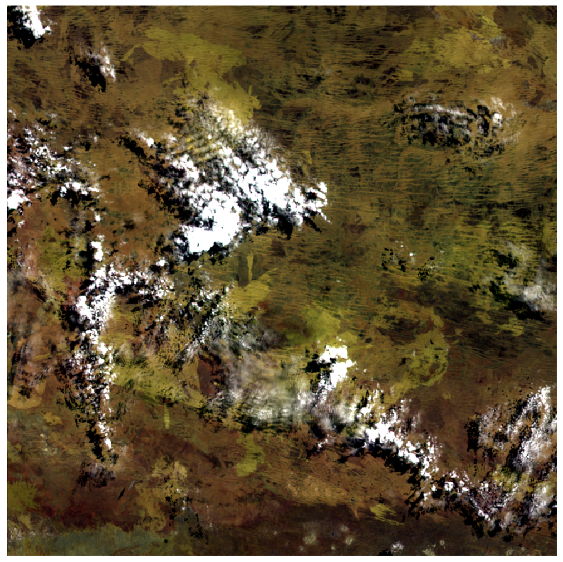
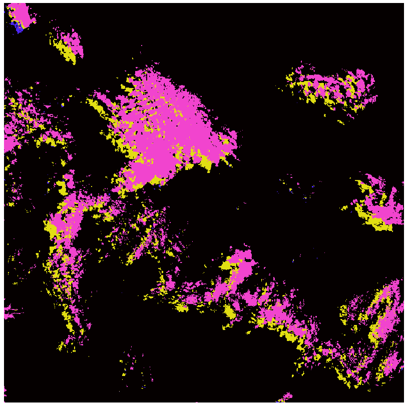
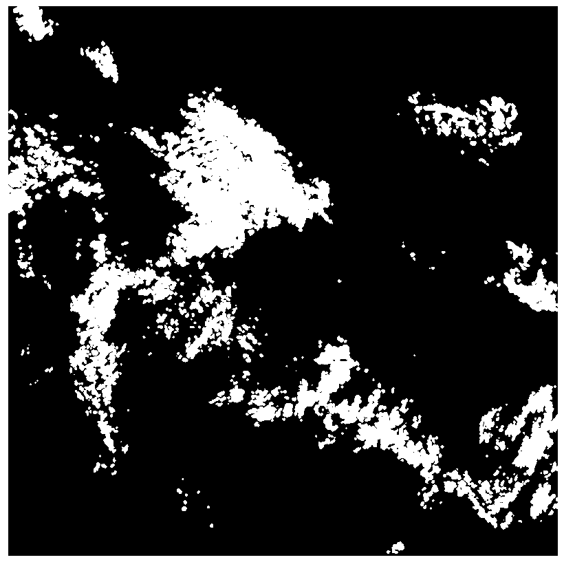
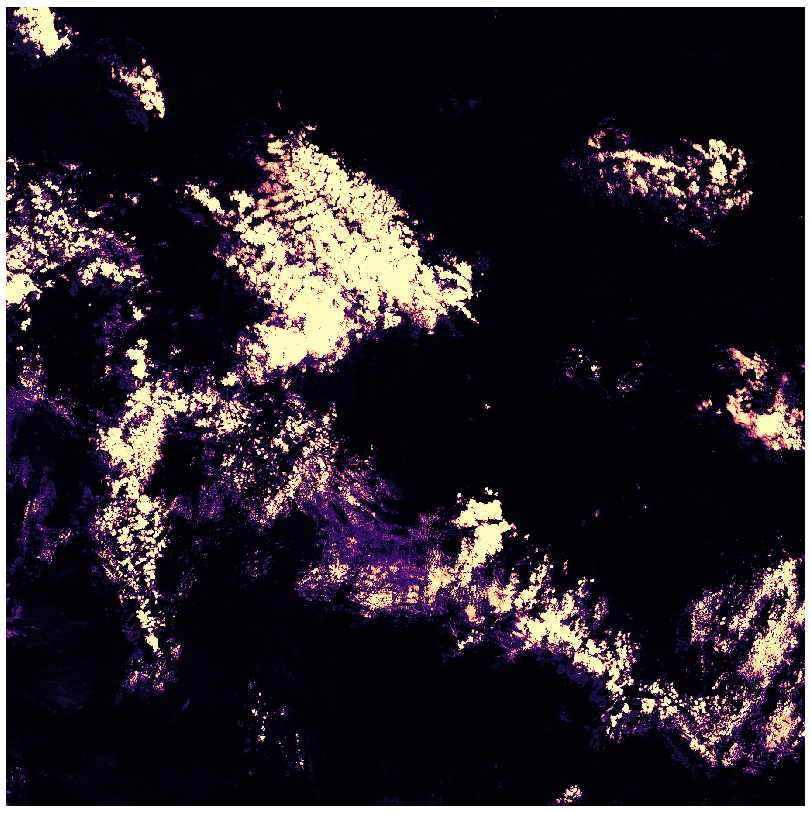
Figure 1. (A) Surface Reflectance (Sentinel-2A) image; (B) Fmask (purple: cloud, yellow: cloud shadow); (C) s2cloudless mask (white: cloud, black: clear); (D) s2cloudless probability.
Terminology for satellite, solar and sensing geometries
Zenith The point in the sky or celestial sphere directly above a point of interest (in this case, the point being imaged on Earth).
Solar zenith (degrees) The angle between the zenith and the centre of the sun’s disc.
Solar azimuth (degrees) The angle of the sun’s position from true north; i.e. the angle between true north and a vertical circle passing through the sun and the point being imaged on Earth.
Satellite view or satellite zenith (degrees) The angle between the zenith and the satellite.
Satellite azimuth (degrees) The angle of the satellite’s position from true north; i.e. the angle between true north and a vertical circle passing through the satellite and the point being imaged on Earth.
Incident angle (degrees) The angle between a ray incident on a surface and the line perpendicular to the surface at the point of incidence.
Exiting angle (degrees) The angle between a ray reflected from a surface and the line perpendicular to the surface at the point of emergence.
Azimuthal incident (degrees) The angle between true north and the incident direction in the slope geometry.
Azimuthal exiting (degrees) The angle between true north and the exiting direction in the slope geometry.
Relative azimuth (degrees) The relative azimuth angle between the sun and view directions.
Relative slope (degrees) The relative azimuth angle between the incident and exiting directions in the slope geometry.
Timedelta (seconds) The time from satellite apogee (the point of orbit at which the satellite is furthest from the Earth).
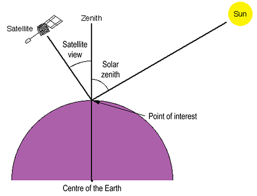
Figure 2. Zenith angles. Image modified from Support to Aviation Control Service (2011).
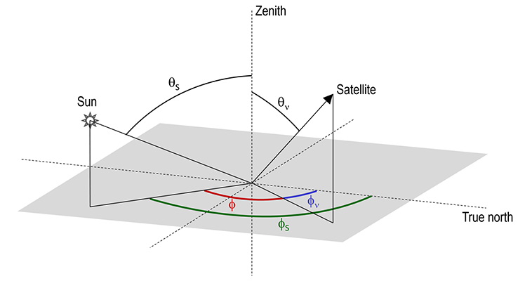
Figure 3. Zenith and azimuth angles. θs = solar zenith; θν = satellite view; Φs = solar azimuth (green); Φν = satellite azimuth (blue); Φ = relative azimuth (red). Image modified from Hudson et al. (2006).
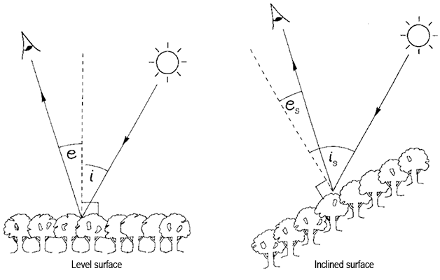
Figure 4. Incident (i) and exiting (e) angles for a level and inclined surface. Image modified from Dymond and Shepherd (1999).
The Fmask algorithm
Fmask allows you to have pre-classified image content for use within applications. This can include:
additional confidence metrics in image content classifiers
pre-labelled data for machine learning classifiers
pixel screening for cloud and cloud shadow
on-the-fly mapping applications for water and snow.
The result of the Fmask algorithm contains mutually exclusive classified pixels, and the numerical schema for the pixels are as follows:
0 = null
1 = clear
2 = cloud
3 = cloud shadow
4 = snow
5 = water.
The s2cloudless algorithm
Sentinel Hub’s cloud detection algorithm is a specialised machine-learning-based algorithm for the Sentinel-2 MSI sensors. This algorithm includes both a per-pixel cloud probability layer (i.e. probability of each satellite pixel being covered by cloud), and an integer cloud mask derived from these cloud probabilities. The numerical schema for the integer cloud mask is:
0 = null
1 = clear
2 = cloud.
Contiguity and terrain
The spectrally contiguous pixels which have a valid observation in each spectral band. This is particularly useful for applications undertaking band math, as it allows non-contiguous data to be ignored during the band math evaluation or masked during post-evaluation. The product can be utilised as a strict mask, and the numerical schema for the pixels are as follows:
0 = non-contiguous
1 = contiguous.
The terrain-shaded pixels product can be utilised as a strict mask and exclude pixels that were unobservable by the sun or sensor. The numerical schema for the pixels are as follows:
0 = shaded
1 = not shaded.
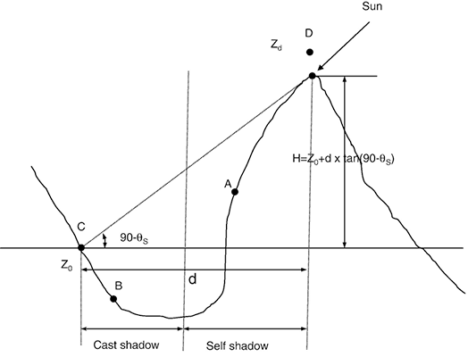
Figure 5. Different types of terrain-shaded pixels. C = point of interest; D = point located along the direction of the sun; 90-θS = solar zenith; Z0 = elevation at location C; Zd = elevation at location D. Image sourced from Li et al. (2012).
Example - Fmask
Some analyses might want to exclude targets that are obscured by cloud or cloud shadow. This is particularly useful for applications looking to harvest statistical information for particular regions of interest, such as field crops, where large swaths of data aren’t required to be loaded into computer memory. Instead, only the regions of interest are loaded, analysed and summarised, reducing computational costs.
The following images represent the surface reflectance image and derived Fmask classification result for visual context. The colours for the Fmask classification are displayed as:
Black = clear
Magenta = cloud
Yellow = cloud shadow
Cyan = snow
Dark blue = water.
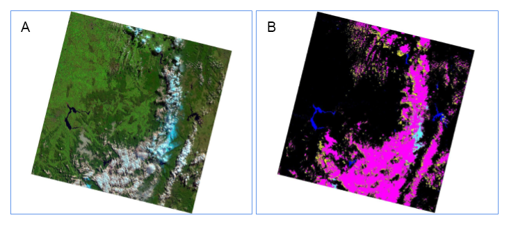
Figure 6. (A) False colour composite; (B) the resulting Fmask classification.
For this product, the Fmask dataset has had the object dilation for the cloud and cloud shadow layers removed. This enables you to customise object dilation to meet your needs for specific applications. For example, one application might work better having a 7-pixel dilation, whereas another might require 5.
You can also choose your own kernel shape and size in which to apply a particular dilation. Dilation can be useful for filling holes within objects and extending the edges of detected objects. It is important to note that small objects (e.g. 1 or 2 pixels in size) will be dilated and become large objects. If this is an undesired outcome, it is best to filter out any small objects prior to applying dilation filters.
For more information on dilation, see:
Other uses of Fmask:
For training data for use with machine learning classifiers Fmask can help refine the result and produce a more accurate classification result. The data can also be combined with other classifiers, creating a confidence metric that users can then filter by. For example, you can filter cloud pixels rated >70% as a combined metric from the combination of cloud classifiers.
For input into a statistical summary It can provide another information product that can be used to indicate the probability of being a particular classified feature. For example, a statistical summary of cloud and/or cloud shadow can highlight pixels that are consistently being detected as a cloud or cloud shadow. As clouds and cloud shadows are non-persistent features, pixels with a high cloud or cloud shadow frequency can be labelled or attributed as highly probable of not being cloud or cloud shadow.
Image format specifications
fmask
Format |
GeoTIFF |
Resolution |
20m |
Datatype |
UInt8 |
Classification ENUM |
0 = null |
Valid data range |
[0,5] |
Tiled with X and Y block sizes |
512x512 |
Compression |
Deflate, Level 9, Predictor 2 |
Pyramids |
Levels: [8,16,32] |
Contrast stretch |
None |
Output CRS |
As specified by source dataset; source is UTM with WGS84 as the datum |
s2cloudless-mask
Format |
GeoTIFF |
Resolution |
60m |
Datatype |
UInt8 |
Classification ENUM |
0 = null |
Valid data range |
[0,2] |
Tiled with X and Y block sizes |
512x512 |
Compression |
Deflate, Level 9, Predictor 2 |
Pyramids |
Levels: [8,16,32] |
Contrast stretch |
None |
Output CRS |
As specified by source dataset; source is UTM with WGS84 as the datum |
s2cloudless-prob
Format |
GeoTIFF |
Resolution |
60m |
Datatype |
Float64 |
No data value |
NaN (IEEE 754) |
Valid data range |
[0,1] |
Tiled with X and Y block sizes |
512x512 |
Compression |
Deflate, Level 9, Predictor 2 |
Pyramids |
Levels: [8,16,32] |
Contrast stretch |
None |
Output CRS |
As specified by source dataset; source is UTM with WGS84 as the datum |
nbart-contiguity
Format |
GeoTIFF |
Resolution |
10m |
Datatype |
UInt8 |
Classification ENUM |
0 = non-contiguous (spectral information not present in each band) |
Valid data range |
[0,1] |
Tiled with X and Y block sizes |
512x512 |
Compression |
Deflate, Level 9, Predictor 2 |
Pyramids |
Levels: [8,16,32] |
Contrast stretch |
None |
Output CRS |
As specified by source dataset; source is UTM with WGS84 as the datum |
combined-terrain-shadow
Format |
GeoTIFF |
Resolution |
20m |
Datatype |
UInt8 |
Classification ENUM |
0 = terrain shadow |
Valid data range |
[0,1] |
Tiled with X and Y block sizes |
512x512 |
Compression |
Deflate, Level 9, Predictor 2 |
Pyramids |
None |
Contrast stretch |
None |
Output CRS |
As specified by source dataset; source is UTM with WGS84 as the datum |
incident-angle, exiting-angle, azimuthal-incident, azimuthal-exiting, relative-azimuth, relative-slope, timedelta
Format |
GeoTIFF |
Resolution |
20m |
No data value |
NaN (IEEE 754) |
Tiled with X and Y block sizes |
512x512 |
Compression |
Deflate, Level 9, Predictor 2 |
Pyramids |
None |
Contrast stretch |
None |
Output CRS |
As specified by source dataset; source is UTM with WGS84 as the datum |
Processing steps
References
Sanchez, A.H., Picoli, M.C.A., Camara, G., Andrade, P.R., Chaves, M.E.D., Lechler, S., Soares, A.R., Marujo, R.F., Simões, R.E.O., Ferreira, K.R. and Queiroz, G.R. (2020). Comparison of Cloud cover detection algorithms on sentinel-2 images of the amazon tropical forest. Remote Sensing, 12(8), 1284.
Accuracy
For information on the accuracy of the algorithms for test locations, see Zhu and Woodcock (2012) and Zhu, Wang and Woodcock (2015).
Limitations
Fmask
Fmask has limitations due to the complex nature of detecting natural phenomena, such as cloud. For example, bright targets, such as beaches, buildings and salt lakes often get mistaken for clouds.
Fmask is designed to be used as an immediate/rapid source of information screening. The idea is that over a temporal period enough observations will be made to form a temporal likelihood. For example, if a feature is consistently being masked as cloud, it is highly probable that it is not cloud. As such, derivative processes can be created to form an information layer containing feature probabilities.
Edges and fringes of clouds tend to be more opaque and can be missed by the cloud detection algorithm. In this instance, applying a morphological dilation will grow the original cloud object and capture edges and fringes of clouds. However, it is important to note that other cloud objects could also be dilated. Be mindful of single-pixel objects that could grow to become large objects. Consider filtering out these small objects prior to analysis.
s2cloudless
Compared to Fmask, one limitation of the s2cloudless algorithm is the lack of cloud shadow detection. Cloud detection without a thermal band in the Sentinel-2 MSI is difficult, so most of the caveats around the interpretation of the Fmask classification also applies here. However, the machine-learning approach offers some advantages over the traditional physics-based approach here, and the cloud probability layer may be utilized to tune the cloud mask to specific applications.
Angular measurement and shadow classification
The Digital Elevation Model (DEM) is used for identifying terrain shadow, as well as producing incident and exiting angles. It is derived from the Shuttle Radar Topography Mission (SRTM) and produced with approximately 30 m resolution. As such, any angular measurements and shadow classifications are limited to the precision of the DEM itself. The DEM is known to be noisy across various locations, so to reduce any potential extrema, a Gaussian smooth is applied prior to analysis.
Quality assurance
The first Cloud Mask Intercomparison eXercise (CMIX) validated the Fmask and the s2cloudless algorithms together with 8 other algorithms on 4 different test datasets. Both performed well (>85% average accuracy) among the single-scene cloud detection algorithms.
The calculation of the satellite and solar positional geometry datasets are largely influenced by the publicly available ephemeris data and whether the satellite has an on-board GPS, as well as the geographical information that resides with the imagery data and the metadata published by the data providers. The code to generate the geometry grids is routinely tested and evaluated for accuracy at >6 decimal places of precision.
Access the data
See it on a map |
Learn how to use DEA Maps |
|
Explore data availability |
Learn how to use the DEA Explorer |
|
Get the data online |
Learn how to access the data via AWS |
|
Code sample |
Learn how to use the DEA Sandbox |
|
Get via web service |
Learn how to use DEA’s web services |
How to access Sentinel-2 data using the Open Data Cube
This product is contained in the Open Data Cube instance managed by Digital Earth Australia (DEA). This simplified process allows you to query data from its sub-products as part of a single query submitted to the database.
Introduction to DEA Surface Reflectance (Sentinel-2, Collection 3)
How to access DEA Maps
To view and access the data interactively via a web map interface:
Visit DEA Maps
Click “Explore map data”
Select “Baseline satellite data” -> “DEA Surface Reflectance (Sentinel-2)”
Click “Add to the map”
Old versions
View previous versions of this data product.
Acknowledgments
This research was undertaken with the assistance of resources from the National Computational Infrastructure (NCI), which is supported by the Australian Government.
Contains modified Copernicus Sentinel data 2015-present.
The authors would like to thank the following organisations:
National Aeronautics and Space Administration (NASA)
Environment Canada
The Commonwealth Scientific and Industrial Research Organisation (CSIRO)
National Oceanic and Atmospheric Administration (NOAA) / Earth System Research Laboratories (ESRL) / Physical Sciences Laboratory (PSD)
The National Geospatial-Intelligence Agency (NGA)
The United States Geological Survey (USGS) / Earth Resources Observation and Science (EROS) Center
Spectral Sciences Inc.
License and copyright
© Commonwealth of Australia (Geoscience Australia).
Released under Creative Commons Attribution 4.0 International Licence.