Introduction to DEA Surface Reflectance (Sentinel-2, Collection 3)

Sign up to the DEA Sandbox to run this notebook interactively from a browser
Compatibility: Notebook currently compatible with both the NCI and DEA Sandbox environments
Products used: ga_s2am_ard_3, ga_s2bm_ard_3

Background

The European Space Agency (ESA) has operated medium resolution satellites - Sentinel-2 series (Sentinel-2A and Sentinel-2B) since 2015. The spectral bands and spatial resolution of Sentinel-2 are similar to those of the Landsat series, but Sentinel-2 has a higher revisit frequency and spatial coverage. A combination of Sentinel-2 and Landsat data can provide good spatial and temporal coverage of the Earth’s surface and provide useful information to monitor environmental resources over time, such as agricultural production and mining activities. However, the raw remotely sensed data received by these satellites in the solar spectral range do not directly characterise the underlying reflectance of surface objects. The data are modified by the atmosphere, variation of solar and sensor positions as well as surface anisotropic conditions. To make accurate comparisons of imagery acquired at different times, seasons and geographic locations, and detect the change of surface, it is necessary to remove/reduce these effects to ensure the data are consistent and can be compared over time.

What the Sentinel-2 products offer

The products below take Sentinel-2A and Sentinel-2B imagery captured over the Australian continent and correct for inconsistencies across land and coastal fringes. The result is accurate and standardised surface reflectance data, which is instrumental in identifying and quantifying environmental change.

The imagery is captured using the Multispectral Instrument (MSI) sensor aboard Sentinel-2A and Sentinel-2B.

These products form a single, cohesive Analysis Ready Data (ARD) package, which allows the analysis of surface reflectance data as is, without the need to apply additional corrections.

Sentinel-2A and Sentinel-2B each contain two sub-products that provide corrections or attribution information:

The resolution is a 10/20/60 m grid based on the ESA Level 1C archive.

This Collection 3 (C3) product and has been created by reprocessing Collection 1 (C1) and making improvements to the processing pipeline and packaging.

Packaging updates include:

Open Data Cube (ODC) eo3 metadata.
metadata includes STAC fields to enable users to filter by fields such as tile ID or cloud cover percentage in applications such as ODC.
additional STAC metadata file in JSON format.
directory structure and file names that are consistent with GA’s Landsat C3 products.

Additional updates include:

upgrading the spectral response function to result in a more accurate product. These new versions include minor updates, slight changes of the central wavelengths for band B02 of S2A and S2B, and band B01 of S2B, along with slight changes of the Full Width Half Maximum (FWHM) for most of the bands.
correction of solar constant errors in the conversion between reflectance and radiance as well as in the atmospheric correction.
an additional cloud mask layer (s2cloudless)
automatic Fmask cloud and shadow buffering turned off for consistency with Landsat Collection 3, and greater flexibility for cloud masking in areas affected by false positive clouds
additional geometric quality assessment (GQA) metadata to enable Sentinel-2 images to be filtered by geometric accuracy
removal of NBAR layers.
reduced spatial resolution of observation attribute layers to 20 m resolution, with the contiguity layer being maintained at 10 m.
BRDF ancillary upgraded from MODIS BRDF C5 to MODIS BRDF C6.
Upgrading from MODTRAN 5.2 to MODTRAN 6.

The introduction of a maturity concept:

The Collection 3 product is comprised of data produced to varying degrees of maturity. The maturity of a dataset is dictated by the quality of the ancillary information used to generate the product. The maturity levels are Near Real Time (NRT), Interim and Final. The maturity level is designated in the filename and in the metadata.

Near Real Time (NRT) is a rapid ARD product produced < 48 hours after image capture.
Interim ARD – If there are extended delays (>18 days) in delivery of inputs to the ARD model, we fall back to interim production until the issue is resolved.
Final ARD - As the higher quality ancillary datasets become available, a “Final” version of the Sentinel 2 ARD data is produced, which replaces the NRT or interim product.

Applications

The development of derivative products to monitor land, inland waterways and coastal features, such as:
- urban growth
- coastal habitats
- mining activities
- agricultural activity (e.g. pastoral, irrigated cropping, rain-fed cropping)
- water extent
The development of refined information products, such as:
- areal units of detected surface water
- areal units of deforestation
- yield predictions of agricultural parcels
Compliance surveys
Emergency management

Note: For more technical information about DEA Surface Reflectance, visit the official Geoscience Australia DEA Surface Reflectance product descriptions for Sentinel-2A and Sentinel-2B.

Description

This notebook will demonstrate how to load, plot and filter DEA Surface Reflectance data using the Open Data Cube software. Topics covered include:

Inspecting the products and measurements available in the datacube
Loading DEA Sentinel-2 Surface Reflectance for an example location (including filtering by dataset maturity)
Plotting Sentinel-2 surface reflectance as RGB images
Loading cloud masked Sentinel-2A and 2B data with “load_ard”
Applying a cloud mask using the new “s2cloudless” cloud mask
Dropping cloudy observations
Advanced: Filtering by metadata to remove poorly georeferenced scenes

Getting started

To run this analysis, run all the cells in the notebook, starting with the “Load packages” cell.

Load packages

Import Python packages that are used for the analysis.

[1]:

import datacube
from datacube.utils import masking
from odc.ui import with_ui_cbk
import matplotlib.pyplot as plt

import sys
sys.path.insert(1, '../Tools/')
from dea_tools.datahandling import load_ard
from dea_tools.plotting import rgb

Connect to the datacube

Connect to the datacube so we can access DEA data.

[2]:

# Connect to the datacube and provide a string to indentify this application and track down problems with database queries
dc = datacube.Datacube(app="DEA_Sentinel2_Surface_Reflectance")

Available products and measurements

List products available in Digital Earth Australia

We can use datacube’s list_products functionality to inspect DEA Sentinel-2 Surface Reflectance products that are available in Digital Earth Australia. The table below shows the product name that we will use to load data, and a brief description of the product.

[3]:

# List Sentinel-2 Surface Reflectance products available in DEA
dc_products = dc.list_products()
dc_products.loc[['ga_s2am_ard_3', 'ga_s2bm_ard_3']]

[3]:

	name	description	license	default_crs	default_resolution
name
ga_s2am_ard_3	ga_s2am_ard_3	Geoscience Australia Sentinel 2A MSI Analysis ...	CC-BY-4.0	EPSG:3577	(-10, 10)
ga_s2bm_ard_3	ga_s2bm_ard_3	Geoscience Australia Sentinel 2B MSI Analysis ...	CC-BY-4.0	EPSG:3577	(-10, 10)

List measurements

We can inspect the contents of each of the DEA Sentinel-2 Surface Reflectance products using datacube’s list_measurements() functionality. The table below lists each of the measurements available in the data. These measurements have prefixes nbart_ and oa_ that represent the two main Sentinel-2 “sub-products” that provide analysis ready surface reflectance data, and additional contextual attributes (for more information, see here and here).

[4]:

dc_measurements = dc.list_measurements()
dc_measurements.loc[['ga_s2am_ard_3']]

[4]:

		name	dtype	units	nodata	aliases	flags_definition	spectral_definition
product	measurement
ga_s2am_ard_3	nbart_coastal_aerosol	nbart_coastal_aerosol	int16	1	-999	[nbart_band01, coastal_aerosol]	NaN	NaN
	nbart_blue	nbart_blue	int16	1	-999	[nbart_band02, blue]	NaN	NaN
	nbart_green	nbart_green	int16	1	-999	[nbart_band03, green]	NaN	NaN
	nbart_red	nbart_red	int16	1	-999	[nbart_band04, red]	NaN	NaN
	nbart_red_edge_1	nbart_red_edge_1	int16	1	-999	[nbart_band05, red_edge_1]	NaN	NaN
	nbart_red_edge_2	nbart_red_edge_2	int16	1	-999	[nbart_band06, red_edge_2]	NaN	NaN
	nbart_red_edge_3	nbart_red_edge_3	int16	1	-999	[nbart_band07, red_edge_3]	NaN	NaN
	nbart_nir_1	nbart_nir_1	int16	1	-999	[nbart_band08, nir_1]	NaN	NaN
	nbart_nir_2	nbart_nir_2	int16	1	-999	[nbart_band8a, nir_2]	NaN	NaN
	nbart_swir_2	nbart_swir_2	int16	1	-999	[nbart_band11, swir_2, swir2]	NaN	NaN
	nbart_swir_3	nbart_swir_3	int16	1	-999	[nbart_band12, swir_3]	NaN	NaN
	oa_fmask	oa_fmask	uint8	1	0	[fmask]	{'fmask': {'bits': [0, 1, 2, 3, 4, 5, 6, 7], '...	NaN
	oa_nbart_contiguity	oa_nbart_contiguity	uint8	1	255	[nbart_contiguity]	{'contiguous': {'bits': [0], 'values': {'0': F...	NaN
	oa_azimuthal_exiting	oa_azimuthal_exiting	float32	1	NaN	[azimuthal_exiting]	NaN	NaN
	oa_azimuthal_incident	oa_azimuthal_incident	float32	1	NaN	[azimuthal_incident]	NaN	NaN
	oa_combined_terrain_shadow	oa_combined_terrain_shadow	uint8	1	255	[combined_terrain_shadow]	NaN	NaN
	oa_exiting_angle	oa_exiting_angle	float32	1	NaN	[exiting_angle]	NaN	NaN
	oa_incident_angle	oa_incident_angle	float32	1	NaN	[incident_angle]	NaN	NaN
	oa_relative_azimuth	oa_relative_azimuth	float32	1	NaN	[relative_azimuth]	NaN	NaN
	oa_relative_slope	oa_relative_slope	float32	1	NaN	[relative_slope]	NaN	NaN
	oa_satellite_azimuth	oa_satellite_azimuth	float32	1	NaN	[satellite_azimuth]	NaN	NaN
	oa_satellite_view	oa_satellite_view	float32	1	NaN	[satellite_view]	NaN	NaN
	oa_solar_azimuth	oa_solar_azimuth	float32	1	NaN	[solar_azimuth]	NaN	NaN
	oa_solar_zenith	oa_solar_zenith	float32	1	NaN	[solar_zenith]	NaN	NaN
	oa_time_delta	oa_time_delta	float32	1	NaN	[time_delta]	NaN	NaN
	oa_s2cloudless_mask	oa_s2cloudless_mask	uint8	1	0	[s2cloudless_mask]	{'s2cloudless_mask': {'bits': [0, 1, 2], 'valu...	NaN
	oa_s2cloudless_prob	oa_s2cloudless_prob	float64	1	NaN	[s2cloudless_prob]	NaN	NaN

Sentinel-2 surface reflectance products have 13 spectral bands which cover the visible, near-infrared and short-wave infrared wavelengths. DEA provides access to 11 of these bands (excluding Band 9 Water Vapour and Band 10 Cirrus).

'Sentinel-2 spectral bands'

The table produced by .list_measurements() also contains important information about the measurement data types, units, nodata value and other technical information about each measurement. For example, aliases (e.g. blue) can be used instead of the official measurement name (e.g. nbart_blue) when loading data (see next step).

Plotting Sentinel-2 surface reflectance

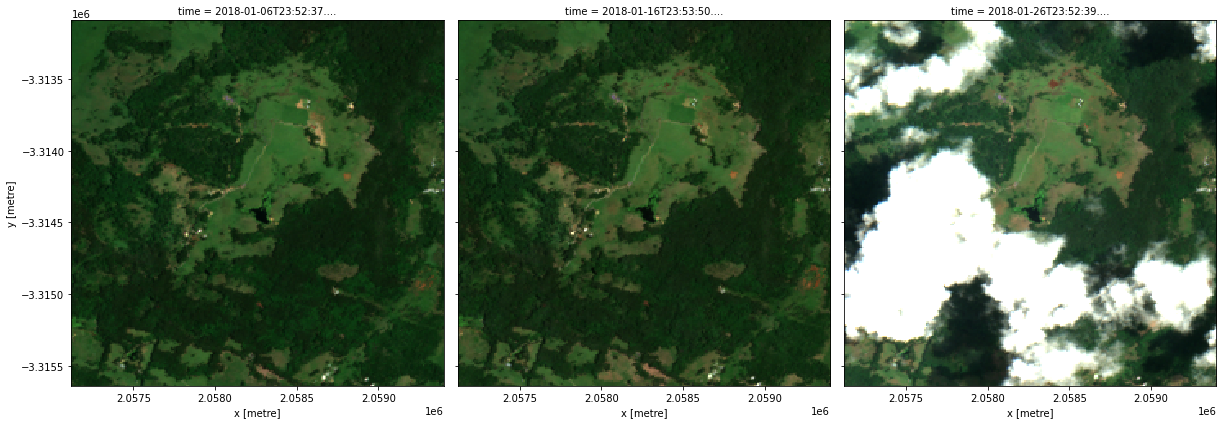
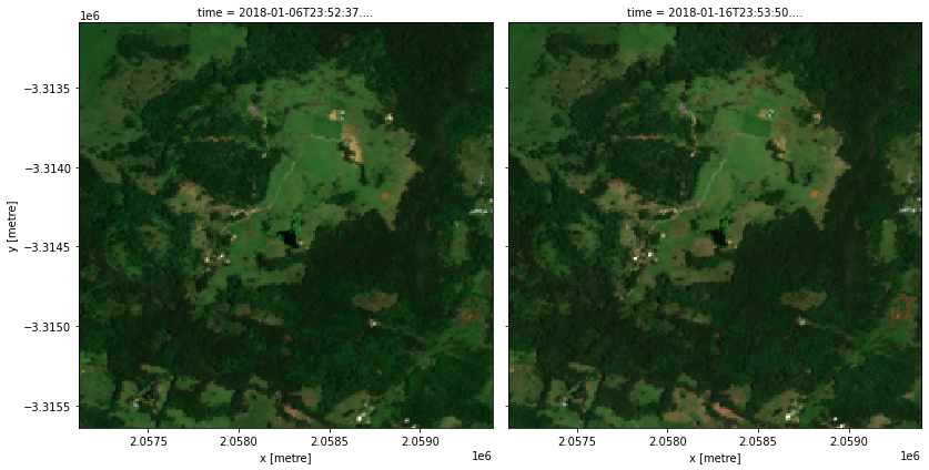
We can use the rgb() plotting function from the dea_tools.plotting Python module to plot the Sentinel-2A images we have loaded for our query region. We can provide vmin and vmax to make sure our colours are shown consistently even when an image is covered in cloud.

[9]:

rgb(ds, col='time', vmin=0, vmax=2000)

../../../_images/notebooks_DEA_products_DEA_Sentinel2_Surface_Reflectance_22_0.png

Loading cloud-masked Sentinel-2A and 2B with `load_ard`

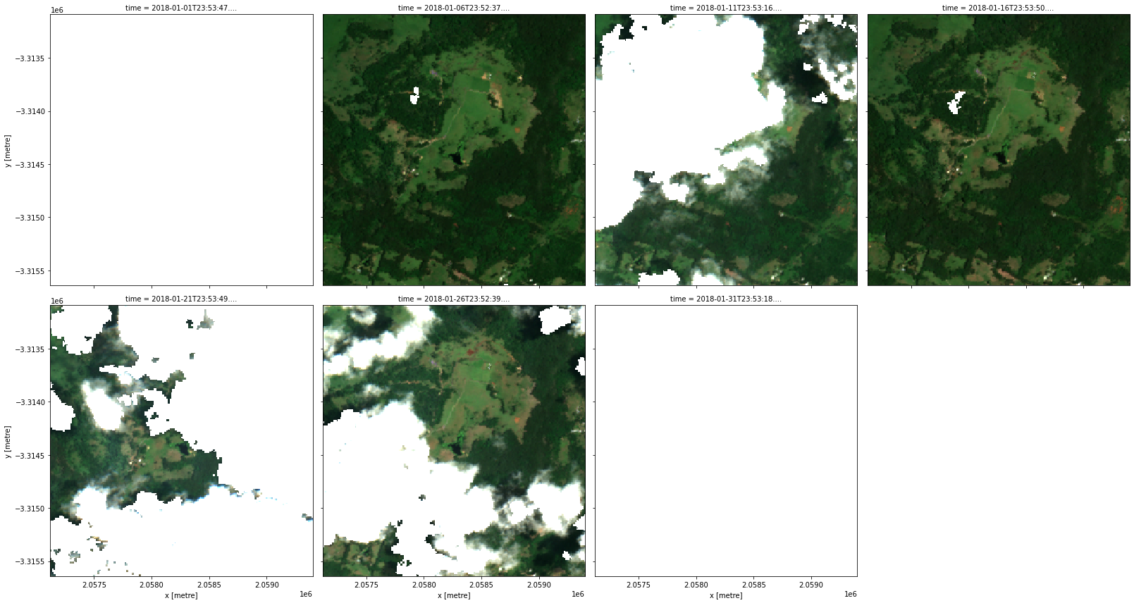
Another option for loading Sentinel-2 data is the load_ard() function, which is a wrapper function around the dc.load() function. This function will load images from both Sentinel-2A and Sentinel-2B, concatenate and sort the observations by time, and apply a cloud mask (by default Fmask; see instructions below to use s2cloudless instead). The result is an analysis-ready dataset.

You can find more information on this function from the Using load ard notebook.

[10]:

ds_ard = load_ard(dc=dc,
                  products=["ga_s2am_ard_3", "ga_s2bm_ard_3"],
                  measurements=bands,
                  **query)

rgb(ds_ard, col='time', vmin=0, vmax=2000)

Finding datasets
    ga_s2am_ard_3
    ga_s2bm_ard_3
Applying fmask pixel quality/cloud mask
Loading 7 time steps

../../../_images/notebooks_DEA_products_DEA_Sentinel2_Surface_Reflectance_25_1.png

Cloud masking using the `s2cloudless` cloud mask

DEA’s Sentinel-2 Surface Reflectance products contain two different cloud masks: the Function of Mask (Fmask) cloud mask, and Sinergise’s Sentinel Hub cloud detector for Sentinel-2 (s2cloudless).

In short, Fmask masks cloud pixels based on their physical characteristics such as brightness, temperature and elevation. This is a problem for Sentinel-2 as it does not have a thermal infrared sensor unlike Landsat-7, 8 and 9, which can lead to potentially serious false positive cloud classifications over bright features like urban areas or coastlines. s2cloudless is a single-scene, pixel-based, machine-learning-based cloud detector trained specifically on Sentinel-2 data, so may produce more accurate cloud classifications on Sentinel-2 data.

Key differences between Fmask and s2cloudless are that additional to clouds, Fmask also classifies cloud shadows, snow and water whereas s2cloudless only classifies clouds. On the other hand, s2cloudless offers a probability layer for clouds whereas the cloud classification from Fmask is discrete (a pixel is either cloud or it is not).

Note: For more information about applying cloud masks using Fmask, see the Masking data notebook, or the Cloud masking section of the DEA Landsat Surface Reflectance notebook.

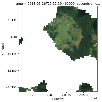
First, let’s extract a single Sentinel-2 image to analyse. By plotting this as a true colour image using rgb, we can see it contains cloud:

[11]:

# Define a new dataset at time index = 2
ds_t2 = ds.isel(time=2)

# Plot as an RGB image:
rgb(ds_t2, vmin=0, vmax=2000)

../../../_images/notebooks_DEA_products_DEA_Sentinel2_Surface_Reflectance_28_0.png

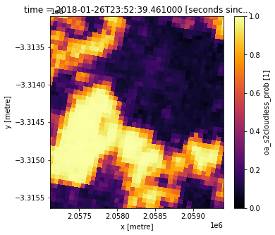
Now let’s view the s2cloudless probability layer! In the image below, bright yellow pixels represent a high probability of cloud.

[12]:

ds_t2.oa_s2cloudless_prob.plot(cmap='inferno', vmin=0, vmax=1.0, aspect=1.1, size=5)

[12]:

<matplotlib.collections.QuadMesh at 0x7fcc380a4ca0>

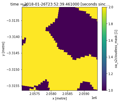
../../../_images/notebooks_DEA_products_DEA_Sentinel2_Surface_Reflectance_30_1.png

s2cloudless uses this cloud probability layer to produce a layer called oa_s2cloudless_mask that contains three possible options: nodata, valid (cloud free) pixels, and clouds:

[13]:

# Display available oa_s2cloudless_mask flags
ds_t2.oa_s2cloudless_mask.flags_definition

[13]:

{'s2cloudless_mask': {'bits': [0, 1, 2],
  'values': {'0': 'nodata', '1': 'valid', '2': 'cloud'},
  'description': 's2cloudless mask'}}

DEA’s oa_s2cloudless_mask layer is calculated using the following steps:

Calculating a moving average of cloud probabilities over a 4 * 60 m pixel window to reduce narrow/small false positives (i.e. ~240 m)
Identifying pixels with a cloud probability of greater than 0.4 (i.e. 40% likelihood of being a cloud)
Dilating these cloud pixels by 2 pixels to conservatively mask out thin cloud edges (i.e. ~120 m)

[14]:

ds_t2.oa_s2cloudless_mask.plot(aspect=1.1, size=5)

[14]:

<matplotlib.collections.QuadMesh at 0x7fcc303c3940>

../../../_images/notebooks_DEA_products_DEA_Sentinel2_Surface_Reflectance_34_1.png

We can use this layer to create a simple cloud mask that we can use to remove cloudy pixels from our Sentinel-2 data by setting them to NaN:

[15]:

# Identify pixels that are "valid" (i.e. containing no cloud). Remember
# 0 = not valid, 1 = no cloud and 2 = cloud, so alternatively you could
# create the same mask using `ds_t2.oa_s2cloudless_mask == 1`
cloud_free_mask = masking.make_mask(ds_t2.oa_s2cloudless_mask,
                                    s2cloudless_mask="valid")

# Keep only the region where there is no cloud
dst2masked = ds_t2.where(cloud_free_mask)

# Plot the cloud masked data:
rgb(dst2masked, vmin=0, vmax=2000)

../../../_images/notebooks_DEA_products_DEA_Sentinel2_Surface_Reflectance_36_0.png

But using the s2cloudless cloud probability layer, we can also customise our cloud masking! For example, we could choose to keep only pixels that have less than a 90% probability of being cloud:

[16]:

# Keep only the pixels where the probabability of cloud is below 90%
dst2probmasked = ds_t2.where(ds_t2.oa_s2cloudless_prob < 0.9)

Next, let’s view the original image, the image after using oa_s2cloudless_mask, and the image after keeping only pixels where oa_s2cloudless_prob < 0.9 respectively:

[17]:

rgb(ds_t2, vmin=0, vmax=2000)
rgb(dst2masked, vmin=0, vmax=2000)
rgb(dst2probmasked, vmin=0, vmax=2000)

../../../_images/notebooks_DEA_products_DEA_Sentinel2_Surface_Reflectance_40_0.png

../../../_images/notebooks_DEA_products_DEA_Sentinel2_Surface_Reflectance_40_1.png

../../../_images/notebooks_DEA_products_DEA_Sentinel2_Surface_Reflectance_40_2.png

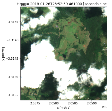
We can see that the last image is difficult to interpret because the masking of NaNs looks like whiter clouds! To work around this, we can manually set the nan pixels to 0 so they appear black.

[18]:

# Manually set the nan regions equal to zero so they don't appear white like clouds!
dst2probmaskedzero = dst2probmasked.where(~dst2probmasked.isnull(), 0)

rgb(dst2probmaskedzero, vmin=0, vmax=2000)

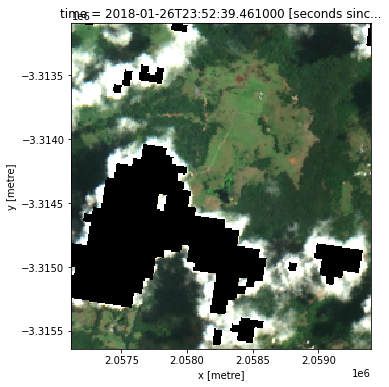
../../../_images/notebooks_DEA_products_DEA_Sentinel2_Surface_Reflectance_42_0.png

Much better!

`s2cloudless` cloud masking with `load_ard`

We can also automatically apply a cloud mask from s2cloudless using the load_ard function introduced above. To do this, provide cloud_mask="s2cloudless" and mask_pixel_quality=True:

[19]:

ds = load_ard(dc=dc,
              products=["ga_s2am_ard_3", "ga_s2bm_ard_3"],
              measurements=bands,
              cloud_mask="s2cloudless",
              mask_pixel_quality=True,
              **query)

rgb(ds, col='time', vmin=0, vmax=2000)

Finding datasets
    ga_s2am_ard_3
    ga_s2bm_ard_3
Applying s2cloudless pixel quality/cloud mask
Loading 7 time steps

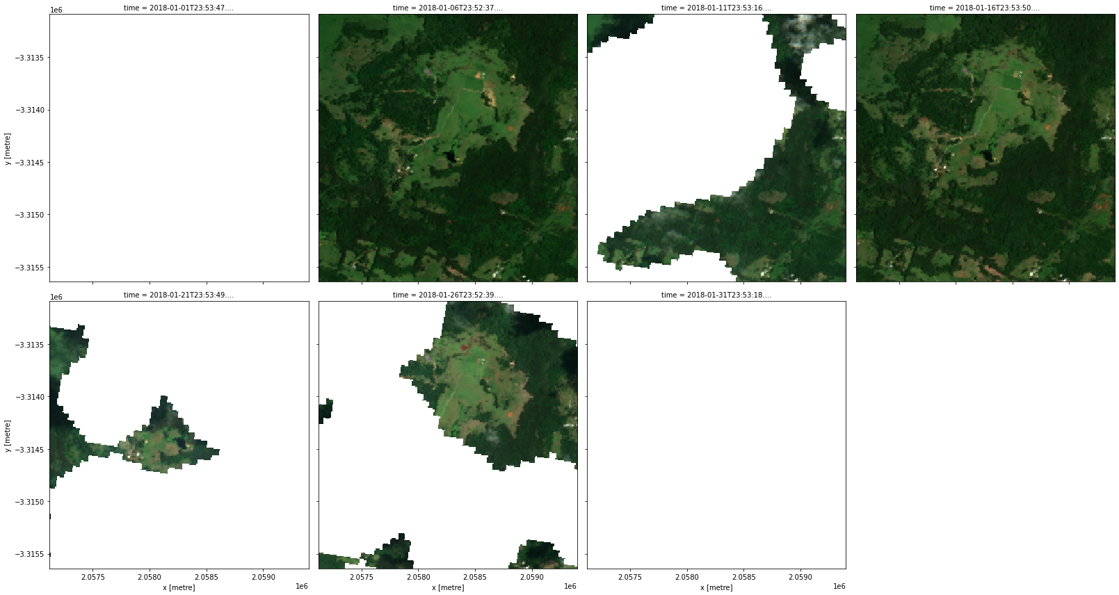
../../../_images/notebooks_DEA_products_DEA_Sentinel2_Surface_Reflectance_45_1.png

Dropping cloudy scenes

When plotting the observations, we can see that some observations are mostly obscured by cloud, leaving very little usable data. To ensure that this does not lead to unrepresentative statistics, we can keep only observations that had (for example) less than 25% cloudy pixels.

[20]:

# Make a new dataset where the value is True where there is cloud and False everywhere else.
# Then take the spatial mean to end up with a cloud percentage for each time index
percent_cloud = (ds.oa_s2cloudless_mask == 2).mean(dim=['x', 'y'])

# Select the observations with a cloud cover percentage less than 25%
ds_noncloudy = ds.sel(time=percent_cloud < 0.25)

If we plot our filtered dataset, we can see that cloudy scenes have now been dropped and we are left with only clear satellite images:

[21]:

# Plot the observations after dropping cloudy scenes
rgb(ds_noncloudy, col='time', vmin=0, vmax=2000)

../../../_images/notebooks_DEA_products_DEA_Sentinel2_Surface_Reflectance_49_0.png

Dropping cloudy scenes using `load_ard`

We can also use load_ard to drop cloudy scenes from our data. To do this we can use the min_gooddata parameter. This works the opposite way to the example above by counting the percent of good quality (e.g. non-cloudy pixels) in each image; to keep images with less than 25% cloud, we can specify min_gooddata=0.75:

[22]:

ds_noncloudy = load_ard(dc=dc,
                        products=["ga_s2am_ard_3", "ga_s2bm_ard_3"],
                        measurements=bands,
                        cloud_mask='s2cloudless',
                        mask_pixel_quality=False,
                        min_gooddata=0.75,
                        **query)

rgb(ds_noncloudy, col='time', vmin=0, vmax=2000)

Finding datasets
    ga_s2am_ard_3
    ga_s2bm_ard_3
Counting good quality pixels for each time step using s2cloudless
Filtering to 2 out of 7 time steps with at least 75.0% good quality pixels
Loading 2 time steps

../../../_images/notebooks_DEA_products_DEA_Sentinel2_Surface_Reflectance_51_1.png

Advanced

Filtering by metadata to remove poorly georeferenced scenes

DEA Sentinel-2 Surface Reflectance data contains a set of extra metadata fields that can be queried to filter data before it is loaded. Searchable metadata fields for a product can be listed using the code below:

[23]:

dataset = dc.find_datasets(product='ga_s2am_ard_3', limit=1)[0]
dir(dataset.metadata)

[23]:

['cloud_cover',
 'creation_dt',
 'creation_time',
 'crs_raw',
 'dataset_maturity',
 'eo_gsd',
 'eo_sun_azimuth',
 'eo_sun_elevation',
 'fmask_clear',
 'fmask_cloud_shadow',
 'fmask_snow',
 'fmask_water',
 'format',
 'gqa_abs_iterative_mean_x',
 'gqa_abs_iterative_mean_xy',
 'gqa_abs_iterative_mean_y',
 'gqa_abs_x',
 'gqa_abs_xy',
 'gqa_abs_y',
 'gqa_cep90',
 'gqa_iterative_mean_x',
 'gqa_iterative_mean_xy',
 'gqa_iterative_mean_y',
 'gqa_iterative_stddev_x',
 'gqa_iterative_stddev_xy',
 'gqa_iterative_stddev_y',
 'gqa_mean_x',
 'gqa_mean_xy',
 'gqa_mean_y',
 'gqa_stddev_x',
 'gqa_stddev_xy',
 'gqa_stddev_y',
 'grid_spatial',
 'id',
 'instrument',
 'label',
 'lat',
 'lon',
 'measurements',
 'platform',
 'product_family',
 'region_code',
 's2cloudless_clear',
 's2cloudless_cloud',
 'sentinel_datastrip_id',
 'sentinel_product_name',
 'sentinel_tile_id',
 'sources',
 'time']

Metadata fields with the prefix gqa_* represent Geometric Quality Assessment metrics, and are particularly useful because Sentinel-2 data has comparatively poor georeferencing (particularly between 2015 and 2017). One of the most useful metadata fields is:

gqa_iterative_mean_xy: An estimate of how accurately a satellite scene is georeferenced, calculated by comparing hundreds of candidate Ground Control Points, then discarding outliers to obtain a more robust estimate. Values are in pixel units based on a 25 metre resolution reference image (i.e. 0.2 = 5 metres)

This parameter can be used to ensure that we only load data that is closely aligned spatially through time. For example, to load only imagery with a geometric accuracy of less than 12.5 m (e.g. 50% of the 25 m reference pixel), we can add gqa_iterative_mean_xy=(0, 0.5) to our dc.load query:

[24]:

ds_geo = dc.load(
    product="ga_s2am_ard_3",
    measurements=["nbart_red"],
    x=(149.10, 149.12),
    y=(-35.29, -35.31),
    time=("2017-09", "2017-10"),
    gqa_iterative_mean_xy=(0, 0.5),
    output_crs="EPSG:3577",
    resolution=(-10, 10),
    group_by="solar_day",
)

Note: If you receive no results when filtering by gqa_* metadata, it may be because these fields had a value of NaN due to no ground control points (GCPs) being available for the location.

Additional information

License: The code in this notebook is licensed under the Apache License, Version 2.0. Digital Earth Australia data is licensed under the Creative Commons by Attribution 4.0 license.

Contact: If you need assistance, please post a question on the Open Data Cube Slack channel or on the GIS Stack Exchange using the open-data-cube tag (you can view previously asked questions here). If you would like to report an issue with this notebook, you can file one on GitHub.

Created: February 2023

Last modified: December 2023

Compatible datacube version:

[25]:

print(datacube.__version__)

1.8.6

Introduction to DEA Surface Reflectance (Sentinel-2, Collection 3)

Background

What the Sentinel-2 products offer

Applications

Description

Getting started

Load packages

Connect to the datacube

Available products and measurements

List products available in Digital Earth Australia

List measurements

Loading Sentinel-2 data

Filtering by dataset maturity

Plotting Sentinel-2 surface reflectance

Loading cloud-masked Sentinel-2A and 2B with `load_ard`

Cloud masking using the `s2cloudless` cloud mask

`s2cloudless` cloud masking with `load_ard`

Dropping cloudy scenes

Dropping cloudy scenes using `load_ard`

Advanced

Filtering by metadata to remove poorly georeferenced scenes

Additional information

Tags

Introduction to DEA Surface Reflectance (Sentinel-2, Collection 3)

Background

What the Sentinel-2 products offer

Applications

Description

Getting started

Load packages

Connect to the datacube

Available products and measurements

List products available in Digital Earth Australia

List measurements

Loading Sentinel-2 data

Filtering by dataset maturity

Plotting Sentinel-2 surface reflectance

Loading cloud-masked Sentinel-2A and 2B with load_ard

Cloud masking using the s2cloudless cloud mask

s2cloudless cloud masking with load_ard

Dropping cloudy scenes

Dropping cloudy scenes using load_ard

Advanced

Filtering by metadata to remove poorly georeferenced scenes

Additional information

Tags

Loading cloud-masked Sentinel-2A and 2B with `load_ard`

Cloud masking using the `s2cloudless` cloud mask

`s2cloudless` cloud masking with `load_ard`

Dropping cloudy scenes using `load_ard`