Introduction to Xarray 
Sign up to the DEA Sandbox to run this notebook interactively from a browser
Compatibility: Notebook currently compatible with both the
NCIandDEA SandboxenvironmentsPrerequisites: Users of this notebook should have a basic understanding of:
How to run a Jupyter notebook
How to work with Numpy
Background
Xarray is a python library which simplifies working with labelled multi-dimension arrays. Xarray introduces labels in the forms of dimensions, coordinates and attributes on top of raw numpy arrays, allowing for more intitutive and concise development. More information about xarray data structures and functions can be found here.
Once you’ve completed this notebook, you may be interested in advancing your xarray skills further, this external notebook introduces more uses of xarray and may help you advance your skills further.
Description
This notebook is designed to introduce users to xarray using Python code in Jupyter Notebooks via JupyterLab.
Topics covered include:
How to use
xarrayfunctions in a Jupyter Notebook cellHow to access
xarraydimensions and metadataUsing indexing to explore multi-dimensional
xarraydataAppliction of built-in
xarrayfunctions such as sum, std and mean
Getting started
To run this notebook, run all the cells in the notebook starting with the “Load packages” cell. For help with running notebook cells, refer back to the Jupyter Notebooks notebook.
Load packages
[1]:
%matplotlib inline

import matplotlib.pyplot as plt
import numpy as np
import xarray as xr
Introduction to xarray
DEA uses xarray as its core data model. To better understand what it is, let’s first do a simple experiment using a combination of plain numpy arrays and Python dictionaries.
Red, NIR and SWIR. These bands are represented as 2-dimensional numpy arrays and the latitude and longitude coordinates for each dimension are represented using 1-dimensional arrays. Finally, we also have some metadata that comes with this image.dictionary.[2]:
# Create fake satellite data
red = np.random.rand(250, 250)
nir = np.random.rand(250, 250)
swir = np.random.rand(250, 250)

# Create some lats and lons
lats = np.linspace(-23.5, -26.0, num=red.shape[0], endpoint=False)
lons = np.linspace(110.0, 112.5, num=red.shape[1], endpoint=False)

# Create metadata
title = "Image of the desert"
date = "2019-11-10"

# Stack into a dictionary
image = {
    "red": red,
    "nir": nir,
    "swir": swir,
    "latitude": lats,
    "longitude": lons,
    "title": title,
    "date": date,
}
All our data is conveniently packed in a dictionary. Now we can use this dictionary to work with the data it contains:
[3]:
# Date of satellite image
print(image["date"])

# Mean of red values
image["red"].mean()
2019-11-10
[3]:
0.5010298934189398
numpy indexes. Wouldn’t it be convenient to be able to select data from the images using the coordinates of the pixels instead of their relative positions?xarray solves! Let’s see how it works:To explore xarray we have a file containing some surface reflectance data extracted from the DEA platform. The object that we get ds is a xarray Dataset, which in some ways is very similar to the dictionary that we created before, but with lots of convenient functionality available.
[4]:
ds = xr.open_dataset("../Supplementary_data/08_Intro_to_xarray/example_netcdf.nc")
ds
[4]:
<xarray.Dataset>
Dimensions:      (time: 12, x: 483, y: 601)
Coordinates:
  * time         (time) datetime64[ns] 2018-01-03T08:31:05 ... 2018-02-27T08:...
  * y            (y) float64 -2.519e+06 -2.519e+06 ... -2.507e+06 -2.507e+06
  * x            (x) float64 2.378e+06 2.378e+06 ... 2.388e+06 2.388e+06
    spatial_ref  int32 6933
Data variables:
    red          (time, y, x) uint16 ...
    green        (time, y, x) uint16 ...
    blue         (time, y, x) uint16 ...
Attributes:
    crs:           EPSG:6933
grid_mapping: spatial_ref- time: 12
- x: 483
- y: 601
- time(time)datetime64[ns]2018-01-03T08:31:05 ... 2018-02-...
array(['2018-01-03T08:31:05.000000000', '2018-01-08T08:34:01.000000000', '2018-01-13T08:30:41.000000000', '2018-01-18T08:30:42.000000000', '2018-01-23T08:33:58.000000000', '2018-01-28T08:30:20.000000000', '2018-02-07T08:30:53.000000000', '2018-02-12T08:31:43.000000000', '2018-02-17T08:23:09.000000000', '2018-02-17T08:35:40.000000000', '2018-02-22T08:34:52.000000000', '2018-02-27T08:31:36.000000000'], dtype='datetime64[ns]') - y(y)float64-2.519e+06 ... -2.507e+06
- units :
- metre
- resolution :
- 20.0
- crs :
- EPSG:6933
array([-2519270., -2519250., -2519230., ..., -2507310., -2507290., -2507270.])
- x(x)float642.378e+06 2.378e+06 ... 2.388e+06
- units :
- metre
- resolution :
- 20.0
- crs :
- EPSG:6933
array([2378390., 2378410., 2378430., ..., 2387990., 2388010., 2388030.])
- spatial_ref()int32...
- spatial_ref :
- PROJCS["WGS 84 / NSIDC EASE-Grid 2.0 Global",GEOGCS["WGS 84",DATUM["WGS_1984",SPHEROID["WGS 84",6378137,298.257223563,AUTHORITY["EPSG","7030"]],AUTHORITY["EPSG","6326"]],PRIMEM["Greenwich",0,AUTHORITY["EPSG","8901"]],UNIT["degree",0.0174532925199433,AUTHORITY["EPSG","9122"]],AUTHORITY["EPSG","4326"]],PROJECTION["Cylindrical_Equal_Area"],PARAMETER["standard_parallel_1",30],PARAMETER["central_meridian",0],PARAMETER["false_easting",0],PARAMETER["false_northing",0],UNIT["metre",1,AUTHORITY["EPSG","9001"]],AXIS["Easting",EAST],AXIS["Northing",NORTH],AUTHORITY["EPSG","6933"]]
- grid_mapping_name :
- lambert_cylindrical_equal_area
array(6933, dtype=int32)
- red(time, y, x)uint16...
- units :
- 1
- nodata :
- 0
- crs :
- EPSG:6933
- grid_mapping :
- spatial_ref
[3483396 values with dtype=uint16]
- green(time, y, x)uint16...
- units :
- 1
- nodata :
- 0
- crs :
- EPSG:6933
- grid_mapping :
- spatial_ref
[3483396 values with dtype=uint16]
- blue(time, y, x)uint16...
- units :
- 1
- nodata :
- 0
- crs :
- EPSG:6933
- grid_mapping :
- spatial_ref
[3483396 values with dtype=uint16]
- crs :
- EPSG:6933
- grid_mapping :
- spatial_ref
Xarray dataset structure
A Dataset can be seen as a dictionary structure packing up the data, dimensions and attributes. Variables in a Dataset object are called DataArrays and they share dimensions with the higher level Dataset. The figure below provides an illustrative example:
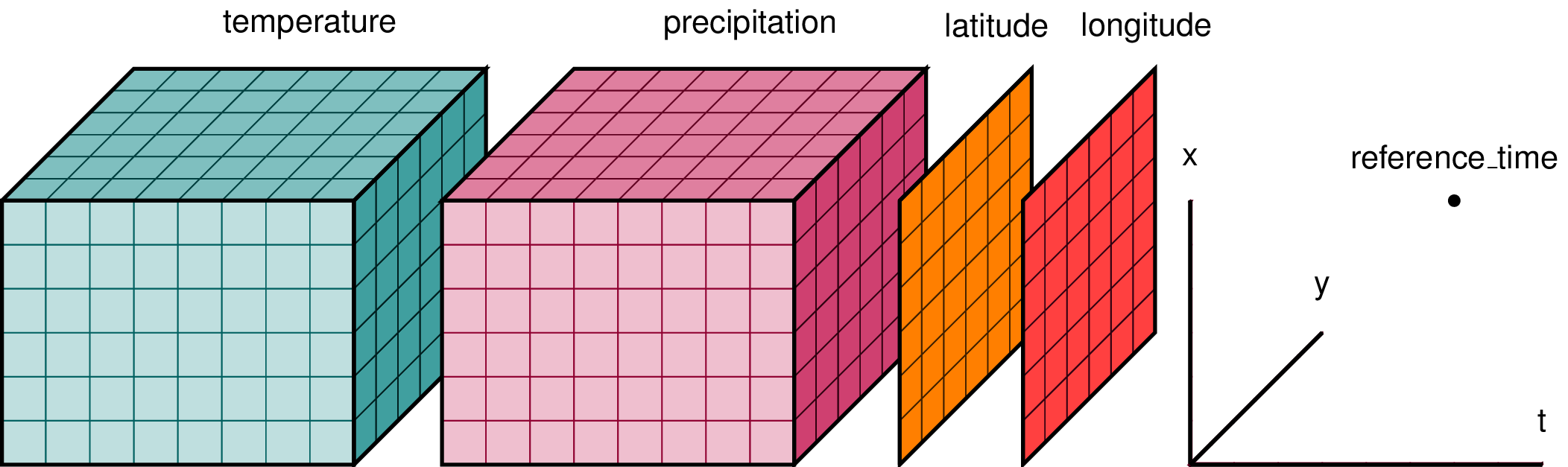
To access a variable we can access as if it were a Python dictionary, or using the . notation, which is more convenient.
[5]:
ds["green"]

# Or alternatively:
ds.green
[5]:
<xarray.DataArray 'green' (time: 12, y: 601, x: 483)>
[3483396 values with dtype=uint16]
Coordinates:
  * time         (time) datetime64[ns] 2018-01-03T08:31:05 ... 2018-02-27T08:...
  * y            (y) float64 -2.519e+06 -2.519e+06 ... -2.507e+06 -2.507e+06
  * x            (x) float64 2.378e+06 2.378e+06 ... 2.388e+06 2.388e+06
    spatial_ref  int32 6933
Attributes:
    units:         1
    nodata:        0
    crs:           EPSG:6933
grid_mapping: spatial_ref- time: 12
- y: 601
- x: 483
- ...
[3483396 values with dtype=uint16]
- time(time)datetime64[ns]2018-01-03T08:31:05 ... 2018-02-...
array(['2018-01-03T08:31:05.000000000', '2018-01-08T08:34:01.000000000', '2018-01-13T08:30:41.000000000', '2018-01-18T08:30:42.000000000', '2018-01-23T08:33:58.000000000', '2018-01-28T08:30:20.000000000', '2018-02-07T08:30:53.000000000', '2018-02-12T08:31:43.000000000', '2018-02-17T08:23:09.000000000', '2018-02-17T08:35:40.000000000', '2018-02-22T08:34:52.000000000', '2018-02-27T08:31:36.000000000'], dtype='datetime64[ns]') - y(y)float64-2.519e+06 ... -2.507e+06
- units :
- metre
- resolution :
- 20.0
- crs :
- EPSG:6933
array([-2519270., -2519250., -2519230., ..., -2507310., -2507290., -2507270.])
- x(x)float642.378e+06 2.378e+06 ... 2.388e+06
- units :
- metre
- resolution :
- 20.0
- crs :
- EPSG:6933
array([2378390., 2378410., 2378430., ..., 2387990., 2388010., 2388030.])
- spatial_ref()int326933
- spatial_ref :
- PROJCS["WGS 84 / NSIDC EASE-Grid 2.0 Global",GEOGCS["WGS 84",DATUM["WGS_1984",SPHEROID["WGS 84",6378137,298.257223563,AUTHORITY["EPSG","7030"]],AUTHORITY["EPSG","6326"]],PRIMEM["Greenwich",0,AUTHORITY["EPSG","8901"]],UNIT["degree",0.0174532925199433,AUTHORITY["EPSG","9122"]],AUTHORITY["EPSG","4326"]],PROJECTION["Cylindrical_Equal_Area"],PARAMETER["standard_parallel_1",30],PARAMETER["central_meridian",0],PARAMETER["false_easting",0],PARAMETER["false_northing",0],UNIT["metre",1,AUTHORITY["EPSG","9001"]],AXIS["Easting",EAST],AXIS["Northing",NORTH],AUTHORITY["EPSG","6933"]]
- grid_mapping_name :
- lambert_cylindrical_equal_area
array(6933, dtype=int32)
- units :
- 1
- nodata :
- 0
- crs :
- EPSG:6933
- grid_mapping :
- spatial_ref
Dimensions are also stored as numeric arrays that we can easily access:
[6]:
ds["time"]

# Or alternatively:
ds.time
[6]:
<xarray.DataArray 'time' (time: 12)>
array(['2018-01-03T08:31:05.000000000', '2018-01-08T08:34:01.000000000',
       '2018-01-13T08:30:41.000000000', '2018-01-18T08:30:42.000000000',
       '2018-01-23T08:33:58.000000000', '2018-01-28T08:30:20.000000000',
       '2018-02-07T08:30:53.000000000', '2018-02-12T08:31:43.000000000',
       '2018-02-17T08:23:09.000000000', '2018-02-17T08:35:40.000000000',
       '2018-02-22T08:34:52.000000000', '2018-02-27T08:31:36.000000000'],
      dtype='datetime64[ns]')
Coordinates:
  * time         (time) datetime64[ns] 2018-01-03T08:31:05 ... 2018-02-27T08:...
spatial_ref int32 6933- time: 12
- 2018-01-03T08:31:05 2018-01-08T08:34:01 ... 2018-02-27T08:31:36
array(['2018-01-03T08:31:05.000000000', '2018-01-08T08:34:01.000000000', '2018-01-13T08:30:41.000000000', '2018-01-18T08:30:42.000000000', '2018-01-23T08:33:58.000000000', '2018-01-28T08:30:20.000000000', '2018-02-07T08:30:53.000000000', '2018-02-12T08:31:43.000000000', '2018-02-17T08:23:09.000000000', '2018-02-17T08:35:40.000000000', '2018-02-22T08:34:52.000000000', '2018-02-27T08:31:36.000000000'], dtype='datetime64[ns]') - time(time)datetime64[ns]2018-01-03T08:31:05 ... 2018-02-...
array(['2018-01-03T08:31:05.000000000', '2018-01-08T08:34:01.000000000', '2018-01-13T08:30:41.000000000', '2018-01-18T08:30:42.000000000', '2018-01-23T08:33:58.000000000', '2018-01-28T08:30:20.000000000', '2018-02-07T08:30:53.000000000', '2018-02-12T08:31:43.000000000', '2018-02-17T08:23:09.000000000', '2018-02-17T08:35:40.000000000', '2018-02-22T08:34:52.000000000', '2018-02-27T08:31:36.000000000'], dtype='datetime64[ns]') - spatial_ref()int326933
- spatial_ref :
- PROJCS["WGS 84 / NSIDC EASE-Grid 2.0 Global",GEOGCS["WGS 84",DATUM["WGS_1984",SPHEROID["WGS 84",6378137,298.257223563,AUTHORITY["EPSG","7030"]],AUTHORITY["EPSG","6326"]],PRIMEM["Greenwich",0,AUTHORITY["EPSG","8901"]],UNIT["degree",0.0174532925199433,AUTHORITY["EPSG","9122"]],AUTHORITY["EPSG","4326"]],PROJECTION["Cylindrical_Equal_Area"],PARAMETER["standard_parallel_1",30],PARAMETER["central_meridian",0],PARAMETER["false_easting",0],PARAMETER["false_northing",0],UNIT["metre",1,AUTHORITY["EPSG","9001"]],AXIS["Easting",EAST],AXIS["Northing",NORTH],AUTHORITY["EPSG","6933"]]
- grid_mapping_name :
- lambert_cylindrical_equal_area
array(6933, dtype=int32)
Metadata is referred to as attributes and is internally stored under .attrs, but the same convenient . notation applies to them.
[7]:
ds.attrs["crs"]

# Or alternatively:
ds.crs
[7]:
'EPSG:6933'
DataArrays store their data internally as multidimensional numpy arrays. But these arrays contain dimensions or labels that make it easier to handle the data. To access the underlaying numpy array of a DataArray we can use the .values notation.
[8]:
arr = ds.green.values

type(arr), arr.shape
[8]:
(numpy.ndarray, (12, 601, 483))
Indexing
Xarray offers two different ways of selecting data. This includes the isel() approach, where data can be selected based on its index (like numpy).
[9]:
print(ds.time.values)

ss = ds.green.isel(time=0)
ss
['2018-01-03T08:31:05.000000000' '2018-01-08T08:34:01.000000000'
 '2018-01-13T08:30:41.000000000' '2018-01-18T08:30:42.000000000'
 '2018-01-23T08:33:58.000000000' '2018-01-28T08:30:20.000000000'
 '2018-02-07T08:30:53.000000000' '2018-02-12T08:31:43.000000000'
 '2018-02-17T08:23:09.000000000' '2018-02-17T08:35:40.000000000'
 '2018-02-22T08:34:52.000000000' '2018-02-27T08:31:36.000000000']
[9]:
<xarray.DataArray 'green' (y: 601, x: 483)>
array([[1214, 1232, 1406, ..., 3436, 4252, 4300],
       [1214, 1334, 1378, ..., 2006, 2602, 4184],
       [1274, 1340, 1554, ..., 2436, 1858, 1890],
       ...,
       [1142, 1086, 1202, ..., 1096, 1074, 1092],
       [1188, 1258, 1190, ..., 1058, 1138, 1138],
       [1152, 1134, 1074, ..., 1086, 1116, 1100]], dtype=uint16)
Coordinates:
    time         datetime64[ns] 2018-01-03T08:31:05
  * y            (y) float64 -2.519e+06 -2.519e+06 ... -2.507e+06 -2.507e+06
  * x            (x) float64 2.378e+06 2.378e+06 ... 2.388e+06 2.388e+06
    spatial_ref  int32 6933
Attributes:
    units:         1
    nodata:        0
    crs:           EPSG:6933
grid_mapping: spatial_ref- y: 601
- x: 483
- 1214 1232 1406 1314 1394 1334 1208 ... 1032 1134 1088 1086 1116 1100
array([[1214, 1232, 1406, ..., 3436, 4252, 4300], [1214, 1334, 1378, ..., 2006, 2602, 4184], [1274, 1340, 1554, ..., 2436, 1858, 1890], ..., [1142, 1086, 1202, ..., 1096, 1074, 1092], [1188, 1258, 1190, ..., 1058, 1138, 1138], [1152, 1134, 1074, ..., 1086, 1116, 1100]], dtype=uint16) - time()datetime64[ns]2018-01-03T08:31:05
array('2018-01-03T08:31:05.000000000', dtype='datetime64[ns]') - y(y)float64-2.519e+06 ... -2.507e+06
- units :
- metre
- resolution :
- 20.0
- crs :
- EPSG:6933
array([-2519270., -2519250., -2519230., ..., -2507310., -2507290., -2507270.])
- x(x)float642.378e+06 2.378e+06 ... 2.388e+06
- units :
- metre
- resolution :
- 20.0
- crs :
- EPSG:6933
array([2378390., 2378410., 2378430., ..., 2387990., 2388010., 2388030.])
- spatial_ref()int326933
- spatial_ref :
- PROJCS["WGS 84 / NSIDC EASE-Grid 2.0 Global",GEOGCS["WGS 84",DATUM["WGS_1984",SPHEROID["WGS 84",6378137,298.257223563,AUTHORITY["EPSG","7030"]],AUTHORITY["EPSG","6326"]],PRIMEM["Greenwich",0,AUTHORITY["EPSG","8901"]],UNIT["degree",0.0174532925199433,AUTHORITY["EPSG","9122"]],AUTHORITY["EPSG","4326"]],PROJECTION["Cylindrical_Equal_Area"],PARAMETER["standard_parallel_1",30],PARAMETER["central_meridian",0],PARAMETER["false_easting",0],PARAMETER["false_northing",0],UNIT["metre",1,AUTHORITY["EPSG","9001"]],AXIS["Easting",EAST],AXIS["Northing",NORTH],AUTHORITY["EPSG","6933"]]
- grid_mapping_name :
- lambert_cylindrical_equal_area
array(6933, dtype=int32)
- units :
- 1
- nodata :
- 0
- crs :
- EPSG:6933
- grid_mapping :
- spatial_ref
Or the sel() approach, used for selecting data based on its dimension of label value.
[10]:
ss = ds.green.sel(time="2018-01-08")
ss
[10]:
<xarray.DataArray 'green' (time: 1, y: 601, x: 483)>
array([[[1270, 1280, ..., 4228, 3950],
        [1266, 1332, ..., 3880, 4372],
        ...,
        [1172, 1180, ..., 1154, 1190],
        [1242, 1204, ..., 1192, 1170]]], dtype=uint16)
Coordinates:
  * time         (time) datetime64[ns] 2018-01-08T08:34:01
  * y            (y) float64 -2.519e+06 -2.519e+06 ... -2.507e+06 -2.507e+06
  * x            (x) float64 2.378e+06 2.378e+06 ... 2.388e+06 2.388e+06
    spatial_ref  int32 6933
Attributes:
    units:         1
    nodata:        0
    crs:           EPSG:6933
grid_mapping: spatial_ref- time: 1
- y: 601
- x: 483
- 1270 1280 1324 1346 1334 1360 1206 ... 1126 1228 1158 1158 1192 1170
array([[[1270, 1280, ..., 4228, 3950], [1266, 1332, ..., 3880, 4372], ..., [1172, 1180, ..., 1154, 1190], [1242, 1204, ..., 1192, 1170]]], dtype=uint16) - time(time)datetime64[ns]2018-01-08T08:34:01
array(['2018-01-08T08:34:01.000000000'], dtype='datetime64[ns]')
- y(y)float64-2.519e+06 ... -2.507e+06
- units :
- metre
- resolution :
- 20.0
- crs :
- EPSG:6933
array([-2519270., -2519250., -2519230., ..., -2507310., -2507290., -2507270.])
- x(x)float642.378e+06 2.378e+06 ... 2.388e+06
- units :
- metre
- resolution :
- 20.0
- crs :
- EPSG:6933
array([2378390., 2378410., 2378430., ..., 2387990., 2388010., 2388030.])
- spatial_ref()int326933
- spatial_ref :
- PROJCS["WGS 84 / NSIDC EASE-Grid 2.0 Global",GEOGCS["WGS 84",DATUM["WGS_1984",SPHEROID["WGS 84",6378137,298.257223563,AUTHORITY["EPSG","7030"]],AUTHORITY["EPSG","6326"]],PRIMEM["Greenwich",0,AUTHORITY["EPSG","8901"]],UNIT["degree",0.0174532925199433,AUTHORITY["EPSG","9122"]],AUTHORITY["EPSG","4326"]],PROJECTION["Cylindrical_Equal_Area"],PARAMETER["standard_parallel_1",30],PARAMETER["central_meridian",0],PARAMETER["false_easting",0],PARAMETER["false_northing",0],UNIT["metre",1,AUTHORITY["EPSG","9001"]],AXIS["Easting",EAST],AXIS["Northing",NORTH],AUTHORITY["EPSG","6933"]]
- grid_mapping_name :
- lambert_cylindrical_equal_area
array(6933, dtype=int32)
- units :
- 1
- nodata :
- 0
- crs :
- EPSG:6933
- grid_mapping :
- spatial_ref
Slicing data is also used to select a subset of data.
[11]:
ss.x.values[100]
[11]:
2380390.0
[12]:
ss = ds.green.sel(time="2018-01-08", x=slice(2378390, 2380390))
ss
[12]:
<xarray.DataArray 'green' (time: 1, y: 601, x: 101)>
array([[[1270, 1280, ..., 1416, 1290],
        [1266, 1332, ..., 1368, 1274],
        ...,
        [1172, 1180, ..., 1086,  991],
        [1242, 1204, ..., 1019,  986]]], dtype=uint16)
Coordinates:
  * time         (time) datetime64[ns] 2018-01-08T08:34:01
  * y            (y) float64 -2.519e+06 -2.519e+06 ... -2.507e+06 -2.507e+06
  * x            (x) float64 2.378e+06 2.378e+06 2.378e+06 ... 2.38e+06 2.38e+06
    spatial_ref  int32 6933
Attributes:
    units:         1
    nodata:        0
    crs:           EPSG:6933
grid_mapping: spatial_ref- time: 1
- y: 601
- x: 101
- 1270 1280 1324 1346 1334 1360 1206 ... 1080 1058 1060 1030 1019 986
array([[[1270, 1280, ..., 1416, 1290], [1266, 1332, ..., 1368, 1274], ..., [1172, 1180, ..., 1086, 991], [1242, 1204, ..., 1019, 986]]], dtype=uint16) - time(time)datetime64[ns]2018-01-08T08:34:01
array(['2018-01-08T08:34:01.000000000'], dtype='datetime64[ns]')
- y(y)float64-2.519e+06 ... -2.507e+06
- units :
- metre
- resolution :
- 20.0
- crs :
- EPSG:6933
array([-2519270., -2519250., -2519230., ..., -2507310., -2507290., -2507270.])
- x(x)float642.378e+06 2.378e+06 ... 2.38e+06
- units :
- metre
- resolution :
- 20.0
- crs :
- EPSG:6933
array([2378390., 2378410., 2378430., 2378450., 2378470., 2378490., 2378510., 2378530., 2378550., 2378570., 2378590., 2378610., 2378630., 2378650., 2378670., 2378690., 2378710., 2378730., 2378750., 2378770., 2378790., 2378810., 2378830., 2378850., 2378870., 2378890., 2378910., 2378930., 2378950., 2378970., 2378990., 2379010., 2379030., 2379050., 2379070., 2379090., 2379110., 2379130., 2379150., 2379170., 2379190., 2379210., 2379230., 2379250., 2379270., 2379290., 2379310., 2379330., 2379350., 2379370., 2379390., 2379410., 2379430., 2379450., 2379470., 2379490., 2379510., 2379530., 2379550., 2379570., 2379590., 2379610., 2379630., 2379650., 2379670., 2379690., 2379710., 2379730., 2379750., 2379770., 2379790., 2379810., 2379830., 2379850., 2379870., 2379890., 2379910., 2379930., 2379950., 2379970., 2379990., 2380010., 2380030., 2380050., 2380070., 2380090., 2380110., 2380130., 2380150., 2380170., 2380190., 2380210., 2380230., 2380250., 2380270., 2380290., 2380310., 2380330., 2380350., 2380370., 2380390.]) - spatial_ref()int326933
- spatial_ref :
- PROJCS["WGS 84 / NSIDC EASE-Grid 2.0 Global",GEOGCS["WGS 84",DATUM["WGS_1984",SPHEROID["WGS 84",6378137,298.257223563,AUTHORITY["EPSG","7030"]],AUTHORITY["EPSG","6326"]],PRIMEM["Greenwich",0,AUTHORITY["EPSG","8901"]],UNIT["degree",0.0174532925199433,AUTHORITY["EPSG","9122"]],AUTHORITY["EPSG","4326"]],PROJECTION["Cylindrical_Equal_Area"],PARAMETER["standard_parallel_1",30],PARAMETER["central_meridian",0],PARAMETER["false_easting",0],PARAMETER["false_northing",0],UNIT["metre",1,AUTHORITY["EPSG","9001"]],AXIS["Easting",EAST],AXIS["Northing",NORTH],AUTHORITY["EPSG","6933"]]
- grid_mapping_name :
- lambert_cylindrical_equal_area
array(6933, dtype=int32)
- units :
- 1
- nodata :
- 0
- crs :
- EPSG:6933
- grid_mapping :
- spatial_ref
Xarray exposes lots of functions to easily transform and analyse Datasets and DataArrays. For example, to calculate the spatial mean, standard deviation or sum of the green band:
[13]:
print("Mean of green band:", ds.green.mean().values)
print("Standard deviation of green band:", ds.green.std().values)
print("Sum of green band:", ds.green.sum().values)
Mean of green band: 4141.488778766468
Standard deviation of green band: 3775.5536474649584
Sum of green band: 14426445446
Plotting data with Matplotlib
Plotting is also conveniently integrated in the library.
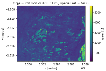
[14]:
ds["green"].isel(time=0).plot()
[14]:
<matplotlib.collections.QuadMesh at 0x7f7684e84400>
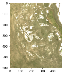
…but we still can do things manually using numpy and matplotlib if you choose:
[15]:
rgb = np.dstack((ds.red.isel(time=0).values,
                 ds.green.isel(time=0).values,
                 ds.blue.isel(time=0).values))
rgb = np.clip(rgb, 0, 2000) / 2000

plt.imshow(rgb);
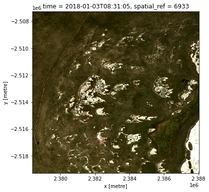
But compare the above to elegantly chaining operations within xarray:
[16]:
ds[["red", "green", "blue"]].isel(time=0).to_array().plot.imshow(robust=True, figsize=(6, 6));
Recommended next steps
For more advanced information about working with Jupyter Notebooks or JupyterLab, you can explore JupyterLab documentation page.
To continue working through the notebooks in this beginner’s guide, the following notebooks are designed to be worked through in the following order:
Introduction to Xarray (this notebook)
Once you have you have completed the above nine tutorials, join advanced users in exploring:
The “Datasets” directory in the repository, where you can explore DEA products in depth.
The “How_to_guides” directory, which contains a recipe book of common techniques and methods for analysing DEA data.
The “Real_world_examples” directory, which provides more complex workflows and analysis case studies.
Additional information
License: The code in this notebook is licensed under the Apache License, Version 2.0. Digital Earth Australia data is licensed under the Creative Commons by Attribution 4.0 license.
Contact: If you need assistance, please post a question on the Open Data Cube Slack channel or on the GIS Stack Exchange using the open-data-cube tag (you can view previously asked questions here). If you would like to report an issue with this notebook, you can file one on
GitHub.
Last modified: December 2023
Tags
Browse all available tags on the DEA User Guide’s `Tags Index <>`__
Tags: sandbox compatible, NCI compatible, xarray, beginner