Using load_ard to load and cloud mask Landsat and Sentinel-2 
Sign up to the DEA Sandbox to run this notebook interactively from a browser
Compatibility: Notebook currently compatible with both the
NCIandDEA SandboxenvironmentsProducts used: ga_ls5t_ard_3, ga_ls7e_ard_3, ga_ls8c_ard_3, ga_ls9c_ard_3, ga_s2am_ard_3, ga_s2bm_ard_3
Description
This notebook demonstrates how to use the load_ard function to import a time series of cloud-free observations from multiple Landsat (i.e. Landsat 5, 7, 8 and 9) or Sentinel-2 (i.e. Sentinel-2A and 2B) satellite products. The function can automatically apply pixel quality masking (e.g. cloud masking) to the input data and return all available data from multiple sensors as a single combined xarray.Dataset.
Optionally, the function can be used to return only observations that contain a minimum proportion of good quality, non-cloudy or shadowed pixels. This can be used to extract visually appealing time series of observations that are not affected by cloud.
The function supports the following Digital Earth Australia products:
Geoscience Australia Landsat Collection 3:
ga_ls5t_ard_3,ga_ls7e_ard_3,ga_ls8c_ard_3,ga_ls9c_ard_3
Geoscience Australia Sentinel-2 Collection 3:
ga_s2am_ard_3,ga_s2bm_ard_3
This notebook demonstrates how to use load_ard to:
Load and combine Landsat 5, 7, 8 and 9 data into a single xarray.Dataset
Filter resulting data to keep only cloud-free observations
Clean and dilate a cloud mask using morphological filtering
Load and combine Sentinel-2A and Sentinel-2B data into a single xarray.Dataset
Advanced: Filter data before loading using metadata and custom functions
Getting started
To run this analysis, run all the cells in the notebook, starting with the “Load packages” cell.
Load packages
[1]:
import datacube
import matplotlib.pyplot as plt

import sys
sys.path.insert(1, '../Tools/')
from dea_tools.datahandling import load_ard
from dea_tools.plotting import rgb
Connect to the datacube
[2]:
dc = datacube.Datacube(app='Using_load_ard')
Loading and combining data from multiple Landsat sensors
The load_ard function can be used to load a single, combined timeseries of cloud-masked data from multiple Digital Earth Australia products or satellite sensors. At its simplest, you can use the function similarly to datacube.load by passing a set of spatiotemporal query parameters (e.g. x, y, time) and load parameters (measurements, output_crs, resolution, group_by etc) directly into the function (see the dc.load documentation for all possible
options). The key difference from dc.load is that load_ard also requires an existing Datacube object, which is passed using the dc parameter. This gives us the flexibilty to load data from development or experimental datacubes.
In the examples below, we load three Landsat bands (red, green and blue) from the four Landsat products (Landsat 5, 7, 8 and 9) by specifying: products=['ga_ls5t_ard_3', 'ga_ls7e_ard_3', 'ga_ls8c_ard_3', 'ga_ls9c_ard_3']:
[3]:
# Load available data from all Landsat satellites
ds = load_ard(dc=dc,
              products=[
                  'ga_ls5t_ard_3', 'ga_ls7e_ard_3', 'ga_ls8c_ard_3',
                  'ga_ls9c_ard_3'
              ],
              measurements=['nbart_green', 'nbart_red', 'nbart_blue'],
              x=(149.06, 149.17),
              y=(-35.27, -35.32),
              time=('2021-06-27', '2021-08-13'),
              output_crs='EPSG:3577',
              resolution=(-30, 30),
              group_by='solar_day')

# Print output data
ds
Finding datasets
    ga_ls5t_ard_3
    ga_ls7e_ard_3
    ga_ls8c_ard_3
    ga_ls9c_ard_3
Applying fmask pixel quality/cloud mask
Loading 12 time steps
CPLReleaseMutex: Error = 1 (Operation not permitted)
[3]:
<xarray.Dataset>
Dimensions:      (time: 12, y: 229, x: 356)
Coordinates:
  * time         (time) datetime64[ns] 2021-06-27T23:50:11.111104 ... 2021-08...
  * y            (y) float64 -3.955e+06 -3.955e+06 ... -3.962e+06 -3.962e+06
  * x            (x) float64 1.544e+06 1.544e+06 ... 1.554e+06 1.554e+06
    spatial_ref  int32 3577
Data variables:
    nbart_green  (time, y, x) float32 926.0 955.0 908.0 ... 576.0 576.0 533.0
    nbart_red    (time, y, x) float32 1.054e+03 1.094e+03 ... 660.0 581.0
    nbart_blue   (time, y, x) float32 775.0 801.0 799.0 ... 322.0 226.0 133.0
Attributes:
    crs:           EPSG:3577
grid_mapping: spatial_refQuery syntax
Often it’s useful to keep our query and load parameters separate so that they can be re-used to load other data in the future. The following example demonstrates how key parameters can be stored in a query dictionary and passed as a single parameter to load_ard:
[4]:
# Create a reusable query
query = {
    'x': (149.06, 149.17),
    'y': (-35.27, -35.32),
    'time': ('2021-06-27', '2021-08-13'),
    'output_crs': 'EPSG:3577',
    'resolution': (-30, 30),
    'group_by': 'solar_day'
}

# Load available data from all three Landsat satellites
ds = load_ard(dc=dc,
              products=[
                  'ga_ls5t_ard_3', 'ga_ls7e_ard_3', 'ga_ls8c_ard_3',
                  'ga_ls9c_ard_3'
              ],
              measurements=['nbart_green', 'nbart_red', 'nbart_blue'],
              **query)

# Print output data
ds
Finding datasets
    ga_ls5t_ard_3
    ga_ls7e_ard_3
    ga_ls8c_ard_3
    ga_ls9c_ard_3
Applying fmask pixel quality/cloud mask
Loading 12 time steps
[4]:
<xarray.Dataset>
Dimensions:      (time: 12, y: 229, x: 356)
Coordinates:
  * time         (time) datetime64[ns] 2021-06-27T23:50:11.111104 ... 2021-08...
  * y            (y) float64 -3.955e+06 -3.955e+06 ... -3.962e+06 -3.962e+06
  * x            (x) float64 1.544e+06 1.544e+06 ... 1.554e+06 1.554e+06
    spatial_ref  int32 3577
Data variables:
    nbart_green  (time, y, x) float32 926.0 955.0 908.0 ... 576.0 576.0 533.0
    nbart_red    (time, y, x) float32 1.054e+03 1.094e+03 ... 660.0 581.0
    nbart_blue   (time, y, x) float32 775.0 801.0 799.0 ... 322.0 226.0 133.0
Attributes:
    crs:           EPSG:3577
grid_mapping: spatial_refCloud masking using mask_pixel_quality
By plotting a time slice from the data we loaded above, you can see an area of white pixels where clouds, shadows or invalid data have been masked out and set to NaN:
[5]:
# Plot single cloud-masked observation
rgb(ds, index=0)
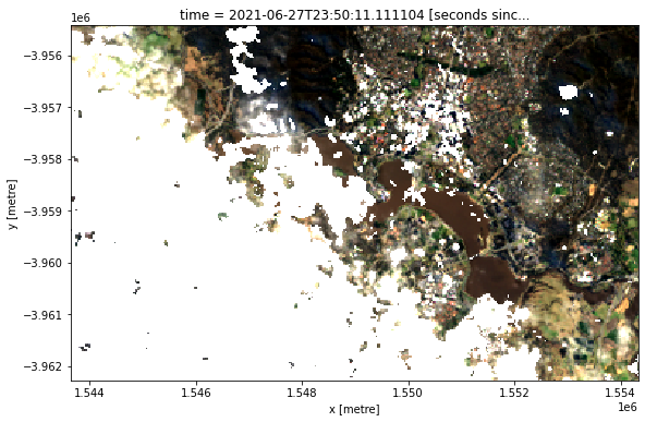
By default, load_ard applies a pixel quality mask to loaded data using the fmask (Function of Mask) cloud mask (this can be changed using the cloud_mask parameter; see Cloud masking with s2cloudless below). The default mask is created based on fmask categories ['valid', 'snow', 'water'] which will preserve non-cloudy or shadowed land, snow and water pixels, and set all invalid, cloudy or shadowy pixels to NaN. This can be customised
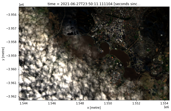
using the fmask_categories parameter. To deactive cloud masking completely, set mask_pixel_quality=False:
[6]:
# Load available data with cloud masking deactivated
ds_cloudy = load_ard(dc=dc,
                     products=[
                         'ga_ls5t_ard_3', 'ga_ls7e_ard_3', 'ga_ls8c_ard_3',
                         'ga_ls9c_ard_3'
                     ],
                     measurements=['nbart_green', 'nbart_red', 'nbart_blue'],
                     mask_pixel_quality=False,
                     **query)

# Plot single observation
rgb(ds_cloudy, index=0)
Finding datasets
    ga_ls5t_ard_3
    ga_ls7e_ard_3
    ga_ls8c_ard_3
    ga_ls9c_ard_3
Loading 12 time steps
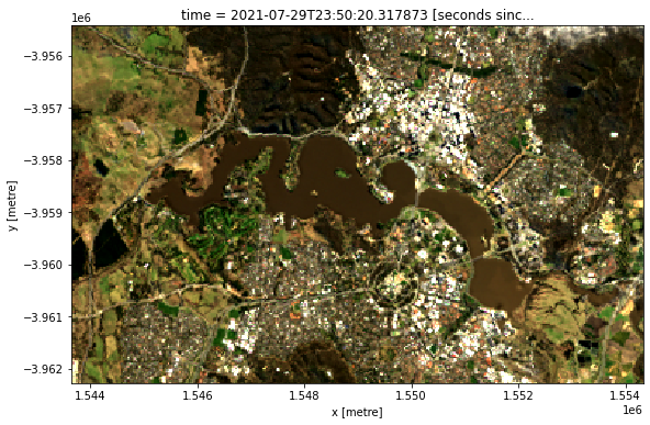
In addition to masking out cloud, load_ard allows you to discard any satellite observation that contains less than a minimum proportion of good quality (e.g. non-cloudy) pixels. This can be used to obtain a time series of only clear, cloud-free observations.
To discard all observations with less than X% good quality pixels, use the min_gooddata parameter. For example, min_gooddata=0.90 will return only observations where less than 10% of pixels contain cloud, cloud shadow or other invalid data, resulting in a smaller number of clear, cloud free images being returned by the function:
[7]:
# Load available data filtered to 90% clear observations
ds_noclouds = load_ard(dc=dc,
                       products=[
                           'ga_ls5t_ard_3', 'ga_ls7e_ard_3', 'ga_ls8c_ard_3',
                           'ga_ls9c_ard_3'
                       ],
                       measurements=['nbart_green', 'nbart_red', 'nbart_blue'],
                       min_gooddata=0.90,
                       mask_pixel_quality=False,
                       **query)

# Plot single observation
rgb(ds_noclouds, index=0)
Finding datasets
    ga_ls5t_ard_3
    ga_ls7e_ard_3
    ga_ls8c_ard_3
    ga_ls9c_ard_3
Counting good quality pixels for each time step using fmask
Filtering to 1 out of 12 time steps with at least 90.0% good quality pixels
Loading 1 time steps
There are significant known limitations to the cloud masking algorithms employed by Sentinel-2 and Landsat. For example, bright objects like buildings and coastlines are commonly mistaken for cloud. We can improve on the false positives detected by Landsat and Sentinel-2’s pixel quality mask by applying binary morphological image processing techniques (e.g.
binary_closing, binary_erosion etc.). The Open Data Cube library odc-algo has a function odc.algo.mask_cleanup that can perform a few of these
operations. Below, we will try to improve the cloud mask by applying a number of these filters.
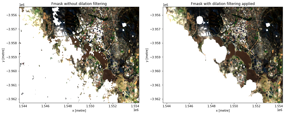
In this example, we use a “morphological opening” operation that first shrinks cloudy areas inward by five pixels, then expands any remaining pixels by five pixels. This operation is useful for removing small, isolated pixels (e.g. false positives caused by bright buildings or sandy coastlines) from our cloud mask, while still preserving the shape of larger clouds. Finally, we apply a “morphological dilation” operation to expand all cloudy areas by five pixels to mask out the thin edges of clouds. Choosing larger values for these parameters (e.g. 10 pixels instead of 5 pixels) will cause load_ard to more aggressively remove noisy pixels, or expand the edges of the cloud mask - you may need to experiment to choose values that work for your application.
Feel free to experiment with the values in filters.
[8]:
# Set the filters to apply
filters = [("opening", 5), ("dilation", 5)]

# Load data
ds_filtered = load_ard(dc=dc,
                       products=[
                           "ga_ls5t_ard_3", "ga_ls7e_ard_3", "ga_ls8c_ard_3",
                           'ga_ls9c_ard_3'
                       ],
                       measurements=['nbart_green', 'nbart_red', 'nbart_blue'],
                       mask_filters=filters,
                       **query)
Finding datasets
    ga_ls5t_ard_3
    ga_ls7e_ard_3
    ga_ls8c_ard_3
    ga_ls9c_ard_3
Applying morphological filters to pixel quality mask: [('opening', 5), ('dilation', 5)]
/home/jovyan/Robbi/dea-notebooks/How_to_guides/../Tools/dea_tools/datahandling.py:487: UserWarning: As of `dea_tools` v0.3.0, pixel quality masks are inverted before being passed to `mask_filters` (i.e. so that good quality/clear pixels are False and poor quality pixels/clouds are True). This means that 'dilation' will now expand cloudy pixels, rather than shrink them as in previous versions.
  warnings.warn(
Applying fmask pixel quality/cloud mask
Loading 12 time steps
Below, you will notice that in the second image the cloud mask is cleaner and less noisy. Buildings in the urban area are removed from the cloud mask while true cloud is more cleanly removed from the dataset.
[9]:
# Plot the data
fig, ax = plt.subplots(1, 2, figsize=(16, 6))
rgb(ds, index=0, ax=ax[0])
rgb(ds_filtered, index=0, ax=ax[1])
ax[0].set_title('Fmask without dilation filtering')
ax[1].set_title('Fmask with dilation filtering applied');
Discarding Landsat 7 SLC-off failure data
On May 31 2003, Landsat 7’s Scan Line Corrector (SLC) that compensated for the satellite’s forward motion failed, introducing linear data gaps in all subsequent Landsat 7 observations. For example, if we plot all our loaded data we can see that some Landsat 7 images contains visible striping:
[10]:
# Plot Landsat data
rgb(ds, col="time")
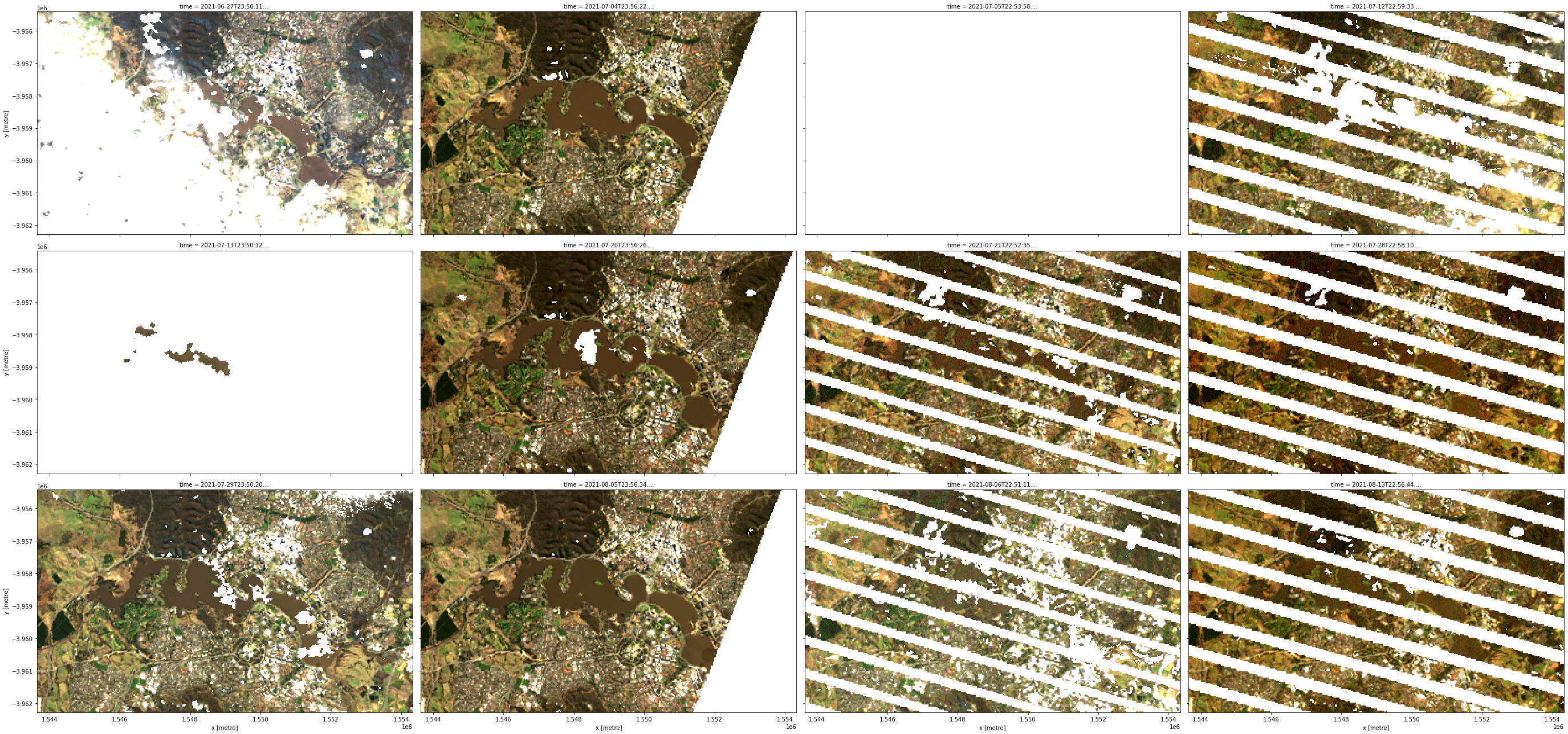
Although this data still contains valuable information, for some applications (e.g. generating clean composites from multiple images) it can be useful to discard Landsat 7 imagery acquired after the SLC failure. This data is known as “SLC-off” data.
This can be achieved using load_ard using the ls7_slc_off. By default this is set to ls7_slc_off=True which will include all SLC-off data. Set to ls7_slc_off=False to discard this data instead; observe that the function now reports that it is ignoring SLC-off observations:
Finding datasets
    ga_ls5t_ard_3
    ga_ls7e_ard_3 (ignoring SLC-off observations)
    ga_ls8c_ard_3
[11]:
# Load available data after discarding Landsat 7 SLC-off data
ds_ls7 = load_ard(dc=dc,
              products=[
                  'ga_ls5t_ard_3', 'ga_ls7e_ard_3', 'ga_ls8c_ard_3',
                  'ga_ls9c_ard_3'
              ],
              measurements=['nbart_green', 'nbart_red', 'nbart_blue'],
              ls7_slc_off=False,
              **query)
Finding datasets
    ga_ls5t_ard_3
    ga_ls7e_ard_3 (ignoring SLC-off observations)
    ga_ls8c_ard_3
    ga_ls9c_ard_3
Applying fmask pixel quality/cloud mask
Loading 6 time steps
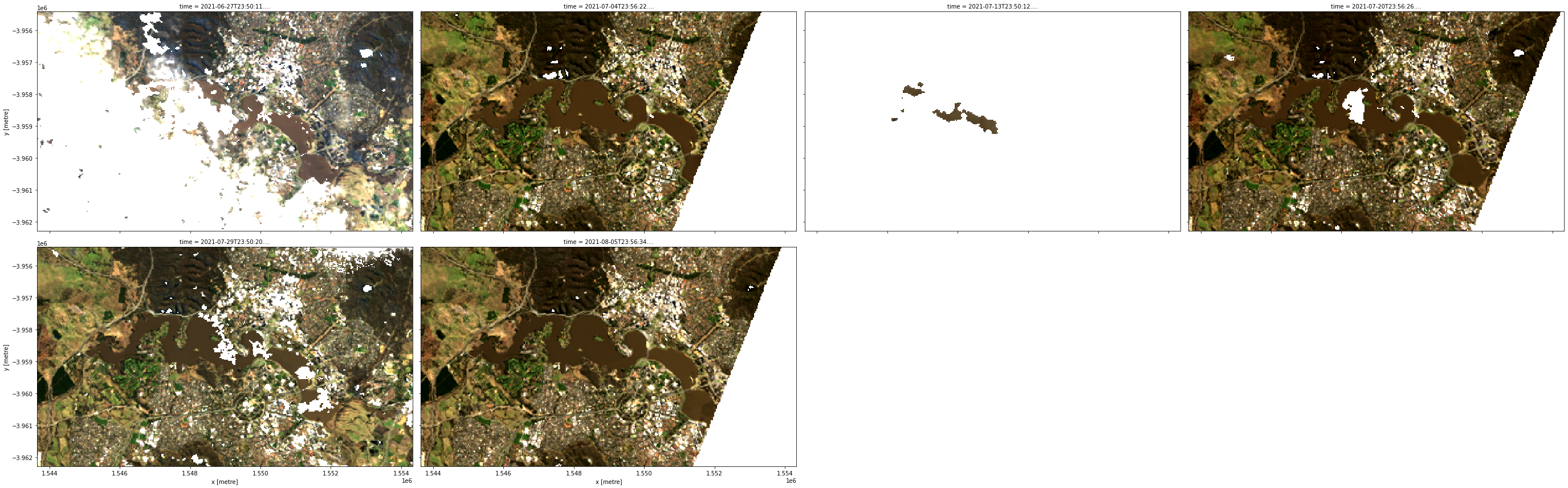
If we plot our data now, we can see that all of the stripey Landsat 7 scenes have now disappeared:
[12]:
# Plot Landsat data
rgb(ds_ls7, col="time")
Loading and combining Sentinel-2A and Sentinel-2B
Data from the Sentinel-2A and Sentinel-2B satellites can also be loaded using load_ard. To do this, we need to specify Sentinel-2 products in place of the Landsat products above.
The query parameter can be re-used to load Sentinel-2 data for the same location and time period.
[13]:
# Load available data from both Sentinel 2 satellites
ds_s2 = load_ard(dc=dc,
                 products=['ga_s2am_ard_3', 'ga_s2bm_ard_3'],
                 measurements=['nbart_green', 'nbart_red', 'nbart_blue'],
                 **query)

# Print output data
ds_s2
Finding datasets
    ga_s2am_ard_3
    ga_s2bm_ard_3
Applying fmask pixel quality/cloud mask
Loading 10 time steps
[13]:
<xarray.Dataset>
Dimensions:      (time: 10, y: 229, x: 356)
Coordinates:
  * time         (time) datetime64[ns] 2021-06-28T00:06:32.739641 ... 2021-08...
  * y            (y) float64 -3.955e+06 -3.955e+06 ... -3.962e+06 -3.962e+06
  * x            (x) float64 1.544e+06 1.544e+06 ... 1.554e+06 1.554e+06
    spatial_ref  int32 3577
Data variables:
    nbart_green  (time, y, x) float32 669.0 684.0 770.0 ... 596.0 582.0 816.0
    nbart_red    (time, y, x) float32 798.0 834.0 814.0 ... 371.0 486.0 835.0
    nbart_blue   (time, y, x) float32 536.0 556.0 564.0 ... 288.0 371.0 486.0
Attributes:
    crs:           EPSG:3577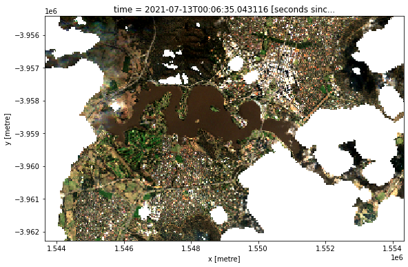
grid_mapping: spatial_refSimilarly to Landsat, cloudy pixels are masked out by default using the Fmask cloud mask:
[14]:
# Plot single observation
rgb(ds_s2, index=3)
Cloud masking with s2cloudless
When working with Sentinel-2 data, users can continue to use Fmask or may try the Sentinel-2 specific cloudmask, s2cloudless, a machine learning cloud mask developed by Sinergise’s Sentinel-Hub.
To apply s2cloudless to your dataset in place of the default Fmask, simply provide cloud_mask='s2cloudless' in your load_ard function call.
The default for s2cloudless will treat ['valid'] pixels as good quality, and set cloudy and nodata pixels to NaN (this can be customised using the s2cloudless_categories parameter):
[15]:
# Load available data from both Sentinel 2 satellites
ds_s2 = load_ard(dc=dc,
                 products=['ga_s2am_ard_3', 'ga_s2bm_ard_3'],
                 measurements=['nbart_green', 'nbart_red', 'nbart_blue'],
                 cloud_mask='s2cloudless',
                 **query)

# Plot single observation
rgb(ds_s2, index=3)
Finding datasets
    ga_s2am_ard_3
    ga_s2bm_ard_3
Applying s2cloudless pixel quality/cloud mask
Loading 10 time steps
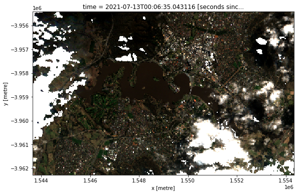
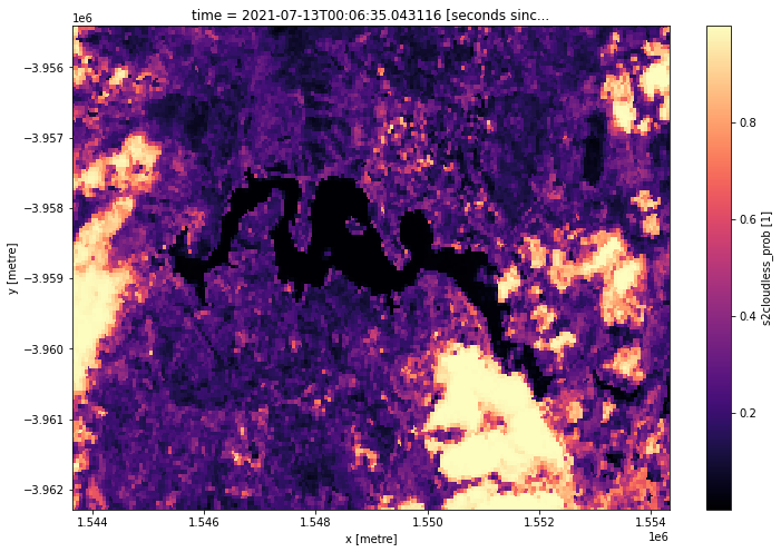
We can also easily load and inspect s2cloudless’s cloud probability layer that gives the likelihood of a pixel containing cloud. Because the load_ard function applies Fmask cloudmasking by default, we can make sure our cloud probability data doesn’t get masked by deactivating cloud masking completely using mask_pixel_quality=False.
[16]:
# Load s2cloudless cloud probabilities from both Sentinel 2 satellites
ds_s2 = load_ard(dc=dc,
                 products=['ga_s2am_ard_3', 'ga_s2bm_ard_3'],
                 measurements=['s2cloudless_prob'],
                 mask_pixel_quality=False,
                 **query)

# Plot single observation
ds_s2.isel(time=3).s2cloudless_prob.plot(size=8, cmap='magma');
Finding datasets
    ga_s2am_ard_3
    ga_s2bm_ard_3
Loading 10 time steps
Note: For more information about cloud masking using
s2cloudless, refer to the DEA Sentinel-2 Surface Reflectance notebook.
Advanced
Filtering data
Using existing dataset metadata
In addition to searching for data by time and location, the load_ard function can filter by any searchable metadata fields available for a product. Searchable metadata options can be viewed under the “Fields” heading on a product’s dataset page in DEA Explorer; for example:
For instance, we could filter to only the highest quality satellite data available by passing in dataset_maturity='final':
[17]:
# Load data with "final" maturity
ds_filtered = load_ard(dc=dc,
                       products=['ga_s2am_ard_3', 'ga_s2bm_ard_3'],
                       measurements=['nbart_green', 'nbart_red', 'nbart_blue'],
                       dataset_maturity='final',
                       **query)
Finding datasets
    ga_s2am_ard_3
    ga_s2bm_ard_3
Applying fmask pixel quality/cloud mask
Loading 10 time steps
Or filter to keep only scenes with high georeferencing accuracy (between 0 and 1 pixel) using gqa_iterative_mean_xy=(0, 1.0):
[18]:
# Load data with high geometric quality assessment accuracy
ds_filtered = load_ard(dc=dc,
                       products=['ga_s2am_ard_3', 'ga_s2bm_ard_3'],
                       measurements=['nbart_green', 'nbart_red', 'nbart_blue'],
                       gqa_iterative_mean_xy=(0, 1.0),
                       **query)
Finding datasets
    ga_s2am_ard_3
    ga_s2bm_ard_3
Applying fmask pixel quality/cloud mask
Loading 9 time steps
Using a custom function
The load_ard function allows you to use Datacube’s powerful dataset_predicate parameter that allows you to filter out satellite observations before they are actually loaded using a custom function. Some examples of where this may be useful include:
Filtering to return data from a specific season (e.g. summer, winter)
Filtering to return data acquired on a particular day of the year
Filtering to return data based on an external dataset (e.g. data acquired during specific climatic conditions such as drought or flood)
A predicate function should take a datacube.model.Dataset object as an input (e.g. as returned from dc.find_datasets(product='ga_ls8c_ard_3', **query)[0]), and return either True or False. For example, a predicate function could be used to return True for only datasets acquired in July:
dataset.time.begin.month == 7
In the example below, we create a simple predicate function that will filter our data to return only satellite data acquired in Julyr:
[19]:
# Simple function that returns True if month is July
def filter_july(dataset):
    return dataset.time.begin.month == 7


# Load data that passes the `filter_july` function
ds_filtered = load_ard(dc=dc,
                       products=['ga_s2am_ard_3', 'ga_s2bm_ard_3'],
                       measurements=['nbart_green', 'nbart_red', 'nbart_blue'],
                       dataset_predicate=filter_july,
                       **query)
Finding datasets
    ga_s2am_ard_3
    ga_s2bm_ard_3
Applying fmask pixel quality/cloud mask
Loading 6 time steps
We can print the time steps returned by load_ard to verify that they now include only July observations (e.g. 2018-07-...):
[20]:
ds_filtered.time
[20]:
<xarray.DataArray 'time' (time: 6)>
array(['2021-07-03T00:06:34.168068000', '2021-07-08T00:06:33.622032000',
       '2021-07-13T00:06:35.043116000', '2021-07-18T00:06:33.968498000',
       '2021-07-23T00:06:35.351606000', '2021-07-28T00:06:33.812679000'],
      dtype='datetime64[ns]')
Coordinates:
  * time         (time) datetime64[ns] 2021-07-03T00:06:34.168068 ... 2021-07...
    spatial_ref  int32 3577
Attributes:
units: seconds since 1970-01-01 00:00:00[21]:
ds_filtered.time.dt.month
[21]:
<xarray.DataArray 'month' (time: 6)>
array([7, 7, 7, 7, 7, 7])
Coordinates:
  * time         (time) datetime64[ns] 2021-07-03T00:06:34.168068 ... 2021-07...
spatial_ref int32 3577Filter to a single season
An example of a predicate function that will return data from a season of interest would look as follows:
def seasonal_filter(dataset, season=[12, 1, 2]):
        #return true if month is in defined season
        return dataset.time.begin.month in season
After applying this predicate function, running the following command demonstrates that our dataset only contains months during the Dec, Jan, Feb period
ds.time.dt.season :

<xarray.DataArray 'season' (time: 37)>
array(['DJF', 'DJF', 'DJF', 'DJF', 'DJF', 'DJF', 'DJF', 'DJF', 'DJF',
       'DJF', 'DJF', 'DJF', 'DJF', 'DJF', 'DJF', 'DJF', 'DJF', 'DJF',
       'DJF', 'DJF', 'DJF', 'DJF', 'DJF', 'DJF', 'DJF', 'DJF', 'DJF',
       'DJF', 'DJF', 'DJF', 'DJF', 'DJF', 'DJF', 'DJF', 'DJF', 'DJF',
       'DJF'], dtype='<U3')
Coordinates:
  * time     (time) datetime64[ns] 2016-01-05T10:27:44.213284 ... 2017-12-26T10:23:43.129624
Lazy loading with Dask
Rather than load data directly - which can take a long time and large amounts of memory - all datacube data can be lazy loaded using Dask. This can be a very useful approach for when you need to load large amounts of data without crashing your analysis, or if you want to subsequently scale your analysis by distributing tasks in parallel across multiple workers.
The load_ard function can be easily adapted to lazily load data rather than loading it into memory by providing a dask_chunks parameter using either the explicit or query syntax. The minimum required to lazily load data is dask_chunks={}, but chunking can also be performed spatially (e.g. dask_chunks={'x': 2048, 'y': 2048}) or by time (e.g. dask_chunks={'time': 1}) depending on the analysis being conducted.
Note: For more information about using Dask, refer to the Parallel processing with Dask notebook.
[22]:
# Lazily load available Sentinel 2 data
ds_dask = load_ard(dc=dc,
                   products=['ga_s2am_ard_3', 'ga_s2bm_ard_3'],
                   measurements=['nbart_green', 'nbart_red', 'nbart_blue'],
                   dask_chunks={'x': 2048, 'y': 2048},
                   **query)

# Print output data
ds_dask
Finding datasets
    ga_s2am_ard_3
    ga_s2bm_ard_3
Applying fmask pixel quality/cloud mask
Returning 10 time steps as a dask array
[22]:
<xarray.Dataset>
Dimensions:      (time: 10, y: 229, x: 356)
Coordinates:
  * time         (time) datetime64[ns] 2021-06-28T00:06:32.739641 ... 2021-08...
  * y            (y) float64 -3.955e+06 -3.955e+06 ... -3.962e+06 -3.962e+06
  * x            (x) float64 1.544e+06 1.544e+06 ... 1.554e+06 1.554e+06
    spatial_ref  int32 3577
Data variables:
    nbart_green  (time, y, x) float32 dask.array<chunksize=(1, 229, 356), meta=np.ndarray>
    nbart_red    (time, y, x) float32 dask.array<chunksize=(1, 229, 356), meta=np.ndarray>
    nbart_blue   (time, y, x) float32 dask.array<chunksize=(1, 229, 356), meta=np.ndarray>
Attributes:
    crs:           EPSG:3577
grid_mapping: spatial_refNote that the data loads almost instantaneously, and that each of the arrays listed under Data variables are now described as dask.arrays. If we inspect one of these dask.arrays, we can view a visualisation of how the data has been broken into small “chunks” of data that can be loaded in parallel:
[23]:
ds_dask.nbart_red
[23]:
<xarray.DataArray 'nbart_red' (time: 10, y: 229, x: 356)>
dask.array<to_float-2c2ce37b, shape=(10, 229, 356), dtype=float32, chunksize=(1, 229, 356), chunktype=numpy.ndarray>
Coordinates:
  * time         (time) datetime64[ns] 2021-06-28T00:06:32.739641 ... 2021-08...
  * y            (y) float64 -3.955e+06 -3.955e+06 ... -3.962e+06 -3.962e+06
  * x            (x) float64 1.544e+06 1.544e+06 ... 1.554e+06 1.554e+06
    spatial_ref  int32 3577
Attributes:
    units:         1
    nodata:        -999
    crs:           EPSG:3577
grid_mapping: spatial_refTo load the data into memory, you can run:
[24]:
ds_dask.compute()
[24]:
<xarray.Dataset>
Dimensions:      (time: 10, y: 229, x: 356)
Coordinates:
  * time         (time) datetime64[ns] 2021-06-28T00:06:32.739641 ... 2021-08...
  * y            (y) float64 -3.955e+06 -3.955e+06 ... -3.962e+06 -3.962e+06
  * x            (x) float64 1.544e+06 1.544e+06 ... 1.554e+06 1.554e+06
    spatial_ref  int32 3577
Data variables:
    nbart_green  (time, y, x) float32 669.0 684.0 770.0 ... 596.0 582.0 816.0
    nbart_red    (time, y, x) float32 798.0 834.0 814.0 ... 371.0 486.0 835.0
    nbart_blue   (time, y, x) float32 536.0 556.0 564.0 ... 288.0 371.0 486.0
Attributes:
    crs:           EPSG:3577
grid_mapping: spatial_refAdditional information
License: The code in this notebook is licensed under the Apache License, Version 2.0. Digital Earth Australia data is licensed under the Creative Commons by Attribution 4.0 license.
Contact: If you need assistance, please post a question on the Open Data Cube Slack channel or on the GIS Stack Exchange using the open-data-cube tag (you can view previously asked questions here). If you would like to report an issue with this notebook, you can file one on
GitHub.
Last modified: December 2023
Compatible datacube version:
[25]:
print(datacube.__version__)
1.8.6
Tags
Tags: sandbox compatible, NCI compatible, load_ard, time series analysis, landsat 5, landsat 7, landsat 8, sentinel 2, cloud masking, cloud filtering, pixel quality, SLC-off, predicate function, Dask, lazy loading