Opening GeoTIFF and NetCDF files with xarray 
Sign up to the DEA Sandbox to run this notebook interactively from a browser
Compatibility: Notebook currently compatible with both the
NCIandDEA Sandboxenvironments
Background
It can be useful open an external raster dataset that you have previously saved to GeoTIFF or NetCDF into a Jupyter notebook in order to conduct further analysis or combine it with other Digital Earth Australia (DEA) data. In this example, we will demonstrate how to load in one or multiple GeoTIFF or NetCDF files originally exported to files from a Landsat-8 time-series into an xarray.Dataset for further analysis.
For advice on exporting raster data, refer to the Exporting GeoTIFFs notebook.
For more information on the xarray and rioxarray functions used:
rioxarray.open_rasterio(https://corteva.github.io/rioxarray/html/rioxarray.html#rioxarray-open-rasterio)xarray.open_dataset(http://xarray.pydata.org/en/stable/generated/xarray.open_dataset.html)xarray.open_mfdataset(http://xarray.pydata.org/en/stable/generated/xarray.open_mfdataset.html)
Description
This notebook shows how to open raster data from file using xarray’s built-in fuctions for handling GeoTIFF and NetCDF files:
Opening single raster files
Opening a single GeoTIFF file
Opening a single NetCDF file
Opening multiple raster files as an
xarray.Datasetwith a time dimensionOpening multiple GeoTIFF files
Opening multiple NetCDF files
Getting started
To run this example, run all the cells in the notebook, starting with the “Load packages” cell.
Load packages
[1]:
%matplotlib inline

import glob
import xarray as xr
import rioxarray

import sys
sys.path.insert(1, '../Tools/')
from dea_tools.datahandling import paths_to_datetimeindex
from dea_tools.plotting import rgb
Opening a single raster file
Define file paths
In the code below we define the locations of the GeoTIFF and NetCDF files that we will open. These files were originally exported from the GA Landsat 8 ga_ls8c_ard_3 product. GeoTIFF files contain a single satellite band (nbart_red), while NetCDF files contain three satellite bands (nbart_red, nbart_green, nbart_blue).
[2]:
geotiff_path = '../Supplementary_data/Opening_GeoTIFFs_NetCDFs/geotiff_red_2018-01-03.tif'
netcdf_path = '../Supplementary_data/Opening_GeoTIFFs_NetCDFs/netcdf_2018-01-03.nc'
Opening a single GeoTIFF
To open a geotiff we use rioxarray.open_rasterio() function which is built around the rasterio Python package. When dealing with extremely large rasters, this function can be used to load data as a Dask array by providing a chunks parameter (e.g. chunks={'x': 1000, 'y': 1000}). This can be useful to reduce memory usage by only loading the specific portion of the raster you are interested in.
[3]:
# Open into an xarray.DataArray
geotiff_da = rioxarray.open_rasterio(geotiff_path)

# Covert our xarray.DataArray into a xarray.Dataset
geotiff_ds = geotiff_da.to_dataset('band')

# Rename the variable to a more useful name
geotiff_ds = geotiff_ds.rename({1: 'red'})
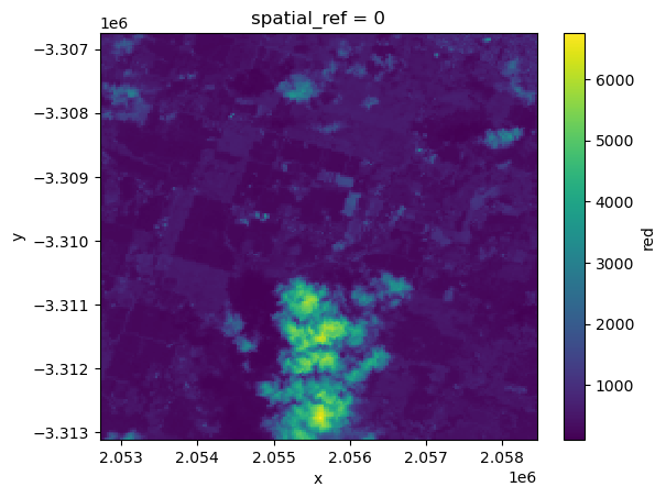
We can plot the data to verify it loaded correctly:
[4]:
geotiff_ds.red.plot()
[4]:
<matplotlib.collections.QuadMesh at 0x7f0ec22d83a0>
Opening a single NetCDF
To open a NetCDF file we can use xarray.open_dataset(). Similarly to the GeoTIFF example above, this function can also be used to open large NetCDF files as Dask arrays by providing a chunks parameter (e.g. chunks={'x': 1000, 'y': 1000}).
[5]:
# Open into an xarray.DataArray
netcdf_ds = xr.open_dataset(netcdf_path)

# We can use 'squeeze' to remove the single time dimension
netcdf_ds = netcdf_ds.squeeze('time')
netcdf_ds
[5]:
<xarray.Dataset>
Dimensions:      (y: 212, x: 191)
Coordinates:
    time         datetime64[ns] 2018-01-03T23:42:39
  * y            (y) float64 -3.307e+06 -3.307e+06 ... -3.313e+06 -3.313e+06
  * x            (x) float64 2.053e+06 2.053e+06 ... 2.058e+06 2.058e+06
Data variables:
    crs          int32 ...
    nbart_red    (y, x) float32 ...
    nbart_green  (y, x) float32 ...
    nbart_blue   (y, x) float32 ...
Attributes:
    date_created:           2019-12-04T16:19:10.855359
    Conventions:            CF-1.6, ACDD-1.3
    history:                NetCDF-CF file created by datacube version '1.7+1...
    geospatial_bounds:      POLYGON ((153.390117090279 -28.8513061571954,153....
    geospatial_bounds_crs:  EPSG:4326
    geospatial_lat_min:     -28.907213271165624
    geospatial_lat_max:     -28.842781641136636
    geospatial_lat_units:   degrees_north
    geospatial_lon_min:     153.39011709027872
    geospatial_lon_max:     153.45973914140396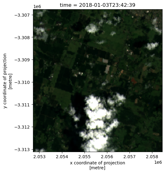
geospatial_lon_units: degrees_eastBecause the NetCDF file we loaded using xarray contain multiple satellite bands (e.g. nbart_red, nbart_green, nbart_blue), we can plot the result in true colour:
[6]:
rgb(netcdf_ds)
Loading multiple files into a single xarray.Dataset
Geospatial time series data is commonly stored as multiple individual files with one time-step per file. These are difficult to use individually, so it can be useful to load multiple files into a single xarray.Dataset prior to analysis. This also allows us to analyse data in a format that is directly compatible with data directly loaded from the Datacube.
Multiple GeoTIFFs
To load multiple GeoTIFF files into a single xarray.Dataset, we first need to obtain a list of the files using the glob package. In the example below, we return a list of any files that match the pattern geotiff_*.tif:
[7]:
geotiff_list = glob.glob('../Supplementary_data/Opening_GeoTIFFs_NetCDFs/geotiff_*.tif')
geotiff_list
[7]:
['../Supplementary_data/Opening_GeoTIFFs_NetCDFs/geotiff_red_2018-01-19.tif',
 '../Supplementary_data/Opening_GeoTIFFs_NetCDFs/geotiff_red_2018-03-24.tif',
 '../Supplementary_data/Opening_GeoTIFFs_NetCDFs/geotiff_red_2018-01-03.tif']
We now read these files using xarray. To ensure each raster is labelled correctly with its time, we can use the helper function paths_to_datetimeindex() from dea_datahandling to extract time information from the file paths we obtained above. We then load and concatenate each dataset along the time dimension using rioxarray.open_rasterio(), convert the resulting xarray.DataArray to a xarray.Dataset, and give the variable a more useful name (red):
[8]:
# Create variable used for time axis
time_var = xr.Variable('time', paths_to_datetimeindex(geotiff_list,
                                                      string_slice=(12, -4)))

# Load in and concatenate all individual GeoTIFFs
geotiffs_da = xr.concat([rioxarray.open_rasterio(i) for i in geotiff_list],
                        dim=time_var)

# Covert our xarray.DataArray into a xarray.Dataset
geotiffs_ds = geotiffs_da.to_dataset('band')

# Rename the variable to a more useful name
geotiffs_ds = geotiffs_ds.rename({1: 'red'})

# Print the output
print(geotiffs_ds)
<xarray.Dataset>
Dimensions:      (time: 3, y: 212, x: 191)
Coordinates:
  * x            (x) float64 2.053e+06 2.053e+06 ... 2.058e+06 2.058e+06
  * y            (y) float64 -3.307e+06 -3.307e+06 ... -3.313e+06 -3.313e+06
    spatial_ref  int64 0
  * time         (time) datetime64[ns] 2018-01-19 2018-03-24 2018-01-03
Data variables:
    red          (time, y, x) int16 902 1307 931 416 544 ... 305 329 332 322 312
Attributes:
    AREA_OR_POINT:  Area
    _FillValue:     0
    scale_factor:   1.0
    add_offset:     0.0
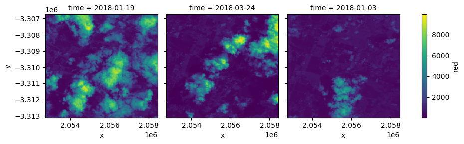
To verify the data was loaded correctly, we can plot it using xarray:
[9]:
geotiffs_ds.red.plot(col='time')
[9]:
<xarray.plot.facetgrid.FacetGrid at 0x7f0ec21c2160>
Multiple NetCDFs
The xarray.open_mfdataset() function can be used to easily load multiple NetCDFs into a single xarray.Dataset. First, we obtain file paths for the files we want to load using glob:
[10]:
netcdf_list = glob.glob('../Supplementary_data/Opening_GeoTIFFs_NetCDFs/netcdf_*.nc')
netcdf_list
[10]:
['../Supplementary_data/Opening_GeoTIFFs_NetCDFs/netcdf_2018-03-24.nc',
 '../Supplementary_data/Opening_GeoTIFFs_NetCDFs/netcdf_2018-01-03.nc',
 '../Supplementary_data/Opening_GeoTIFFs_NetCDFs/netcdf_2018-01-19.nc']
We then load in the NetCDF files using xarray.open_mfdataset. Because the NetCDF file format already contains time information for each dataset, we do not need to set up a time variable like in the previous GeoTIFF example.
[11]:
netcdfs_ds = xr.open_mfdataset(paths=netcdf_list, combine='by_coords')
netcdfs_ds
[11]:
<xarray.Dataset>
Dimensions:      (time: 3, y: 212, x: 191)
Coordinates:
  * time         (time) datetime64[ns] 2018-01-03T23:42:39 ... 2018-03-24T23:...
  * y            (y) float64 -3.307e+06 -3.307e+06 ... -3.313e+06 -3.313e+06
  * x            (x) float64 2.053e+06 2.053e+06 ... 2.058e+06 2.058e+06
Data variables:
    crs          (time) int32 -2147483647 -2147483647 -2147483647
    nbart_red    (time, y, x) float32 dask.array<chunksize=(1, 212, 191), meta=np.ndarray>
    nbart_green  (time, y, x) float32 dask.array<chunksize=(1, 212, 191), meta=np.ndarray>
    nbart_blue   (time, y, x) float32 dask.array<chunksize=(1, 212, 191), meta=np.ndarray>
Attributes:
    date_created:           2019-12-04T16:19:10.855359
    Conventions:            CF-1.6, ACDD-1.3
    history:                NetCDF-CF file created by datacube version '1.7+1...
    geospatial_bounds:      POLYGON ((153.390117090279 -28.8513061571954,153....
    geospatial_bounds_crs:  EPSG:4326
    geospatial_lat_min:     -28.907213271165624
    geospatial_lat_max:     -28.842781641136636
    geospatial_lat_units:   degrees_north
    geospatial_lon_min:     153.39011709027872
    geospatial_lon_max:     153.45973914140396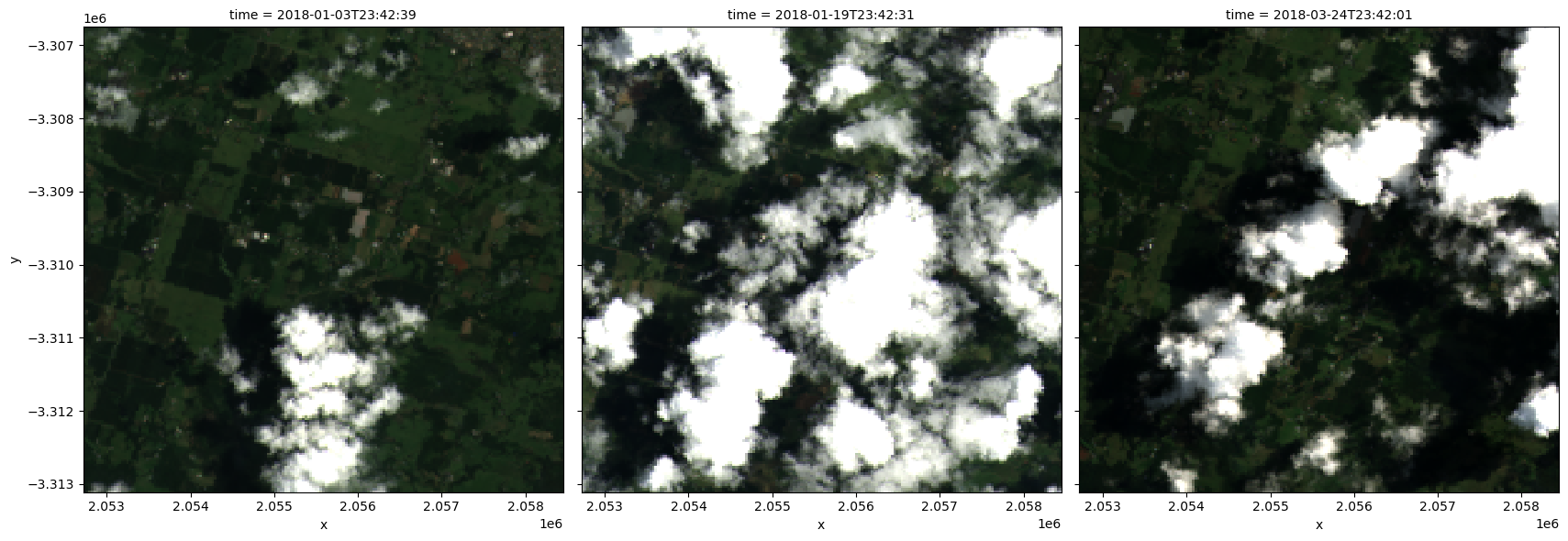
geospatial_lon_units: degrees_eastBecause the NetCDF files we loaded using xarray contain multiple satellite bands (e.g. nbart_red, nbart_green, nbart_blue), we can plot the result in true colour:
[12]:
rgb(netcdfs_ds, col='time', percentile_stretch=(0.0, 0.9))
Additional information
License: The code in this notebook is licensed under the Apache License, Version 2.0. Digital Earth Australia data is licensed under the Creative Commons by Attribution 4.0 license.
Contact: If you need assistance, please post a question on the Open Data Cube Slack channel or on the GIS Stack Exchange using the open-data-cube tag (you can view previously asked questions here). If you would like to report an issue with this notebook, you can file one on
GitHub.
Last modified: December 2023
Tags
Tags: sandbox compatible, NCI compatible, rgb, paths_to_datetimeindex, GeoTIFF, NetCDF, external data, rioxarray.open_rasterio, xarray.open_dataset, xarray.open_mfdataset