Calculating band indices

Sign up to the DEA Sandbox to run this notebook interactively from a browser
Compatibility: Notebook currently compatible with both the DEA Sandbox and NCI environments
Products used: ga_ls8c_ard_3

Background

Remote sensing indices are combinations of spectral bands used to highlight features in the data and the underlying landscape. Using Digital Earth Australia’s archive of analysis-ready satellite data, we can easily calculate a wide range of remote sensing indices that can be used to assist in mapping and monitoring features like vegetation and water consistently through time, or as inputs to machine learning or classification algorithms.

Description

This notebook demonstrates how to:

Calculate an index manually using xarray
Calculate one or multiple indices using the function calculate_indices from dea_tools.bandindices
Calculate indices while dropping original bands from a dataset
Calculate an index in-place without duplicating original data to save memory on large datasets

Getting started

To run this analysis, run all the cells in the notebook, starting with the “Load packages” cell.

Load packages

[1]:

%matplotlib inline

import datacube
import matplotlib.pyplot as plt
import matplotlib.gridspec as gridspec
import numpy as np
import pandas as pd
import xarray as xr

import sys
sys.path.insert(1, '../Tools/')
from dea_tools.datahandling import load_ard
from dea_tools.bandindices import calculate_indices
from dea_tools.plotting import rgb

Connect to the datacube

[2]:

dc = datacube.Datacube(app='Calculating_band_indices')

Create a query and load satellite data

To demonstrate how to compute a remote sensing index, we first need to load in a time series of satellite data for an area. We will use data from the Landsat 8 satellite:

[3]:

# Create a reusable query
query = {
    'x': (149.06, 149.17),
    'y': (-35.27, -35.32),
    'time': ('2020-01', '2020-12'),
    'measurements': [
        'nbart_blue', 'nbart_green', 'nbart_red', 'nbart_nir', 'nbart_swir_1',
        'nbart_swir_2'
    ],
    'output_crs': 'EPSG:3577',
    'resolution': (-30, 30),
    'group_by': 'solar_day'
}

# Load available data from Landsat 8 and filter to retain only times
# with at least 99% good data
ds = load_ard(dc=dc, products=['ga_ls8c_ard_3'], min_gooddata=0.99, **query)

Finding datasets
    ga_ls8c_ard_3
Counting good quality pixels for each time step

CPLReleaseMutex: Error = 1 (Operation not permitted)

Filtering to 5 out of 44 time steps with at least 99.0% good quality pixels
Applying pixel quality/cloud mask
Loading 5 time steps

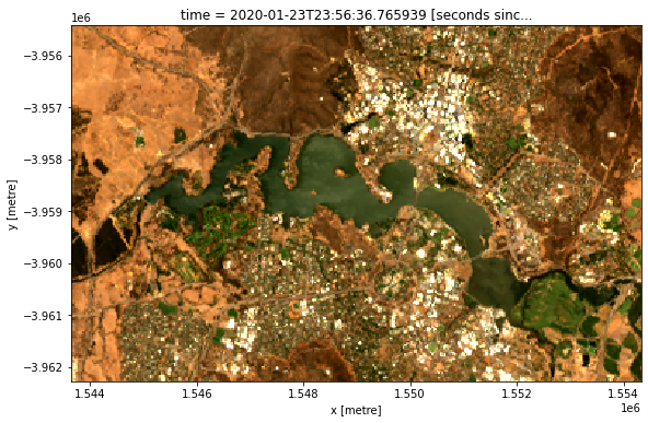
Plot the first image to see what our area looks like

We can use the rgb function to plot the first timestep in our dataset as a true colour RGB image:

[4]:

# Plot as an RGB image
rgb(ds, index=0)

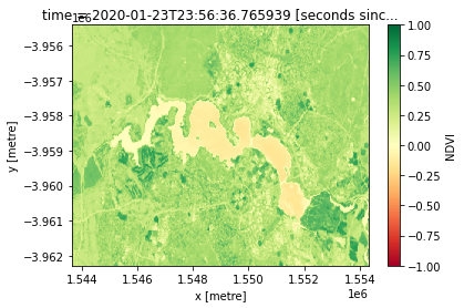
../../../_images/notebooks_How_to_guides_Calculating_band_indices_11_0.png

Calculate an index for this area manually

One of the most commonly used remote sensing indices is the Normalised Difference Vegetation Index or NDVI. This index uses the ratio of the red and near-infrared (NIR) bands to identify live green vegetation. The formula for NDVI is:

\[\begin{split}\begin{aligned} \text{NDVI} & = \frac{(\text{NIR} - \text{Red})}{(\text{NIR} + \text{Red})} \\ \end{aligned}\end{split}\]

When interpreting this index, high values indicate vegetation, and low values indicate soil or water.

[5]:

# Calculate NDVI using the formula above
ds['ndvi'] = (ds.nbart_nir - ds.nbart_red) / (ds.nbart_nir + ds.nbart_red)

# Plot the results for one time step to see what they look like:
ds.ndvi.isel(time=0).plot(vmin=-1, vmax=1, cmap='RdYlGn')

[5]:

<matplotlib.collections.QuadMesh at 0x7fd3c85c21f0>

../../../_images/notebooks_How_to_guides_Calculating_band_indices_13_1.png

In the image above, vegetation shows up as green (NDVI > 0). Sand shows up as yellow (NDVI ~ 0) and water shows up as red (NDVI < 0).

Calculate an index for the same area using `calculate_indices` function

The calculate_indices function provides an easier way to calculate a wide range of remote sensing indices, including:

AWEI_ns (Automated Water Extraction Index,no shadows, Feyisa 2014)
AWEI_sh (Automated Water Extraction Index,shadows, Feyisa 2014)
BAEI (Built-Up Area Extraction Index, Bouzekri et al. 2015)
BAI (Burn Area Index, Martin 1998)
BSI (Bare Soil Index, Rikimaru et al. 2002)
BUI (Built-Up Index, He et al. 2010)
CMR (Clay Minerals Ratio, Drury 1987)
EVI (Enhanced Vegetation Index, Huete 2002)
FMR (Ferrous Minerals Ratio, Segal 1982)
IOR (Iron Oxide Ratio, Segal 1982)
LAI (Leaf Area Index, Boegh 2002)
MNDWI (Modified Normalised Difference Water Index, Xu 1996)
MSAVI (Modified Soil Adjusted Vegetation Index, Qi et al. 1994)
NBI (New Built-Up Index, Jieli et al. 2010)
NBR (Normalised Burn Ratio, Lopez Garcia 1991)
NDBI (Normalised Difference Built-Up Index, Zha 2003)
NDCI (Normalised Difference Chlorophyll Index, Mishra & Mishra, 2012)
NDMI (Normalised Difference Moisture Index, Gao 1996)
NDSI (Normalised Difference Snow Index, Hall 1995)
NDVI (Normalised Difference Vegetation Index, Rouse 1973)
NDWI (Normalised Difference Water Index, McFeeters 1996)
SAVI (Soil Adjusted Vegetation Index, Huete 1988)
TCB (Tasseled Cap Brightness, Crist 1985)
TCG (Tasseled Cap Greeness, Crist 1985)
TCW (Tasseled Cap Wetness, Crist 1985)
WI (Water Index, Fisher 2016)

Using `calculate_indices`, we get the same result:

[6]:

# Calculate NDVI using `calculate indices`
ds_ndvi = calculate_indices(ds, index='NDVI', collection='ga_ls_3')

# Plot the results
ds_ndvi.NDVI.isel(time=0).plot(vmin=-1, vmax=1, cmap='RdYlGn')

[6]:

<matplotlib.collections.QuadMesh at 0x7fd3cbaa7700>

../../../_images/notebooks_How_to_guides_Calculating_band_indices_17_1.png

Note: when using the calculate_indices function, it is important to set the collection parameter correctly. This is because different satellite collections use different names for the same bands, which can lead to invalid results if not accounted for.

For Landsat (i.e. GA Landsat Collection 3), specify collection='ga_ls_3'.

For Sentinel 2 (i.e. GA Sentinel 2 Collection 3), specify collection='ga_s2_3'.

For Landsat geomedian products, specify collection='ga_gm_3'.

Additional information

License: The code in this notebook is licensed under the Apache License, Version 2.0. Digital Earth Australia data is licensed under the Creative Commons by Attribution 4.0 license.

Contact: If you need assistance, please post a question on the Open Data Cube Slack channel or on the GIS Stack Exchange using the open-data-cube tag (you can view previously asked questions here). If you would like to report an issue with this notebook, you can file one on GitHub.

Last modified: December 2023

Compatible datacube version:

[10]:

print(datacube.__version__)

1.8.6

Calculating band indices

Background

Description

Getting started

Load packages

Connect to the datacube

Create a query and load satellite data

Plot the first image to see what our area looks like

Calculate an index for this area manually

Calculate an index for the same area using `calculate_indices` function

Using `calculate_indices`, we get the same result:

Using calculate_indices to calculate multiple indices at once

Dropping original bands from a dataset

Calculating indices in-place to reduce memory usage for large datasets

Additional information

Tags

Calculating band indices

Background

Description

Getting started

Load packages

Connect to the datacube

Create a query and load satellite data

Plot the first image to see what our area looks like

Calculate an index for this area manually

Calculate an index for the same area using calculate_indices function

Using calculate_indices, we get the same result:

Using calculate_indices to calculate multiple indices at once

Dropping original bands from a dataset

Calculating indices in-place to reduce memory usage for large datasets

Additional information

Tags

Calculate an index for the same area using `calculate_indices` function

Using `calculate_indices`, we get the same result: