Reprojecting datacube and raster data

• Sign up to the DEA Sandbox to run this notebook interactively from a browser

• Compatability: Notebook currently compatible with both the NCI and DEA Sandbox environments

• Products used: ga_ls8c_ard_3

• Special requirements: This notebook loads data from an external raster file (canberra_dem_250m.tif) from the Supplementary_data folder of this repository

Background

It is often valuable to combine data from the datacube with other external raster datasets. For example, we may want to use a Digital Elevation Model (DEM) raster as a mask to focus our analysis on satellite data from areas of low or high elevation. However, it can be challenging to combine datasets if they have different extents, resolutions (e.g. 30 m vs. 250 m), or coordinate reference systems (e.g. WGS 84 vs. Australian Albers). To be able to combine these datasets, we need to be able to reproject them into identical spatial grids prior to analysis.

Datacube stores information about the location, resolution and coordinate reference system of a rectangular grid of data using an object called a GeoBox. This GeoBox object is dynamically calculated for data loaded from the datacube and all rasters loaded with rioxarray.open_rasterio using the Open Data Cube Geo / odc-geo package,(provided that import odc.geo.xr is run before the raster is loaded). Datacube functions can use this object to provide a template that can be used to reproject raster and datacube data - either applying this reprojection directly when new data is being loaded, or to reproject existing data that has already been loaded into memory. This makes it straightforward to reproject one dataset into the exact spatial grid of another dataset for further analysis.

Description

This notebook demonstrates how to perform three key reprojection workflows when working with datacube data and external rasters:

1. Loading and reprojecting datacube data to match a raster file using dc.load

2. Reprojecting existing datacube data to match a raster using .odc.reproject()

3. Loading and reprojecting a raster to match datacube data using load_reproject.

---

Getting started

To run this analysis, run all the cells in the notebook, starting with the “Load packages” cell.

Load packages

Import Python packages that are used for the analysis.

import datacube
import xarray as xr
import rioxarray
import odc.geo.xr
import matplotlib.pyplot as plt
from datacube.utils.masking import mask_invalid_data

import sys

sys.path.insert(1, "../Tools/")
from dea_tools.plotting import rgb
from dea_tools.datahandling import load_reproject

Connect to the datacube

Connect to the datacube so we can access DEA data. The app parameter is a unique name for the analysis which is based on the notebook file name.

dc = datacube.Datacube(app="Reprojecting_data")

Loading and reprojecting datacube data to match a raster

Load a raster file

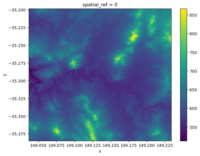
First we load a GeoTIFF raster from file using rioxarray.open_rasterio. The example below loads a single band Digital Elevation Model raster from the Shuttle Radar Topography Mission for the Canberra region (Jarvis et al. 2008) with a low spatial resolution of ~0.002075 decimel degrees (approximately equal to 250 m pixels at the equator) in the WGS 84 (EPSG:4326) coordinate reference system.

# Path to raster file
raster_path = "../Supplementary_data/Reprojecting_data/canberra_dem_250m.tif"

# Load raster, and remove redundant "band" dimension
raster = rioxarray.open_rasterio(raster_path).squeeze("band", drop=True)

If we plot our loaded raster, we can see Canberra’s Lake Burley Griffin in the centre as an area of low elevation (dark pixels), and nearby areas of higher elevation as brighter pixels (e.g. Mt Ainslie, Black Mountain, Red Hill). Note that the raster will appear pixelated due to the large ~250 m pixels:

raster.plot(size=6)

<matplotlib.collections.QuadMesh at 0x7f957fe0d0c0>

GeoBox objects

Now we have loaded our raster dataset, we can inspect its GeoBox object that we will use to allow us to reproject data. The GeoBox can be accessed using the .odc.geobox method. It includes a set of information that together completely define the spatial grid of our data:

• The dimensions (e.g. 95x90) giving the width and height of our data in pixels

• The spatial resolution of our data (e.g. 0.002 degrees)

• The coordinate reference system of our data (e.g. 4326)

raster.odc.geobox

GeoBox

Dimensions

95x90

EPSG

4326

Resolution

0.00207691°

Cell

10px

WKT

GEOGCRS["WGS 84",
    DATUM["World Geodetic System 1984",
        ELLIPSOID["WGS 84",6378137,298.257223563,
            LENGTHUNIT["metre",1]]],
    PRIMEM["Greenwich",0,
        ANGLEUNIT["degree",0.0174532925199433]],
    CS[ellipsoidal,2],
        AXIS["geodetic latitude (Lat)",north,
            ORDER[1],
            ANGLEUNIT["degree",0.0174532925199433]],
        AXIS["geodetic longitude (Lon)",east,
            ORDER[2],
            ANGLEUNIT["degree",0.0174532925199433]],
    ID["EPSG",4326]]

The GeoBox also has a number of useful methods that can be used to view information about the spatial grid of our data. For example, we can inspect the spatial resolution of our data:

raster.odc.geobox.resolution

Resolution(x=0.00207691, y=-0.00207517)

Or obtain information about the data’s spatial extent:

raster.odc.geobox.boundingbox

BoundingBox(left=149.036528545, bottom=-35.384897602, right=149.233835134, top=-35.198132594, crs=CRS('GEOGCS["WGS 84",DATUM["WGS_1984",SPHEROID["WGS 84",6378137,298.257223563,AUTHORITY["EPSG","7030"]],AUTHORITY["EPSG","6326"]],PRIMEM["Greenwich",0,AUTHORITY["EPSG","8901"]],UNIT["degree",0.0174532925199433,AUTHORITY["EPSG","9122"]],AXIS["Latitude",NORTH],AXIS["Longitude",EAST],AUTHORITY["EPSG","4326"]]'))

Note: For more information about GeoBox objects and a complete list of their methods, refer to the datacube documentation.

Load and reproject datacube data

We can now use datacube to load and reproject satellite data to exactly match the coordinate reference system and resolution of our raster data. By specifying like=raster.odc.geobox, we can load datacube data that will be reprojected to match the spatial grid of our raster.

Note: In the current version of datacube, we need to add .compat to our GeoBox object for compatibility reasons. This will not be necessary in the future.

# Load and reproject data from datacube
ds = dc.load(product="ga_ls8c_ard_3",
             measurements=["nbart_red", "nbart_green", "nbart_blue"],
             time=("2019-01-10", "2019-01-15"),
             like=raster.odc.geobox.compat,
             resampling="nearest",
             group_by="solar_day")

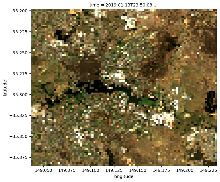
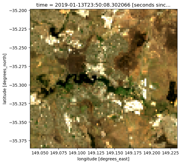
When we plot the result, it should appear similarly pixelated to the low resolution raster we loaded above:

rgb(ds, col='time')

We can also directly compare the geobox of the two datasets to verify they share the same spatial grid:

ds.odc.geobox == raster.odc.geobox

True

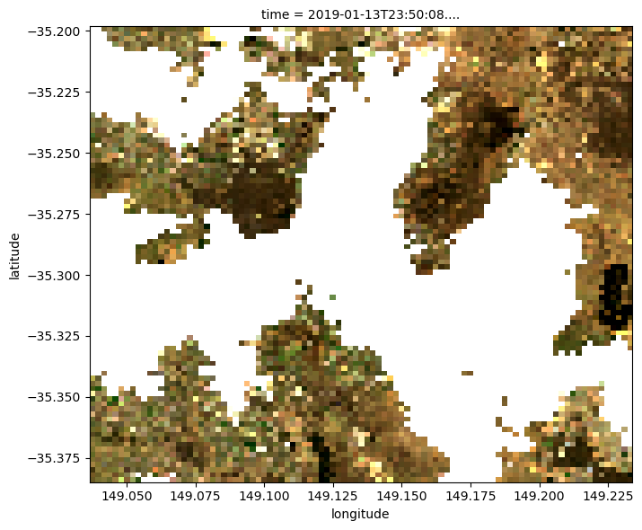
Now that our two datasets share the same spatial grid, we can use our raster as a mask. For example, we can mask out all satellite pixels except those located on hills (e.g. greater than 600 m elevation):

# Identify hilly areas
is_hilly = raster > 600

# Apply mask to set non-hilly areas to `NaN`. We need to use `.data`
# here to use our data as a plain Numpy array as our loaded elevation
# raster uses different coordinates to our satellite data (e.g.
# longitude/latitude vs x/y). This would otherwise prevent us from
# combining them
ds_masked = ds.where(is_hilly.data)

# Plot the masked data
rgb(ds_masked, col="time")

/env/lib/python3.10/site-packages/matplotlib/cm.py:494: RuntimeWarning: invalid value encountered in cast
  xx = (xx * 255).astype(np.uint8)

Reprojecting existing datacube data to match a raster

The example above demonstrated how to load new satellite data from the datacube to match the spatial grid of a raster. However, sometimes we may have already loaded satellite data with a coordinate reference system and resolution that is different from our raster. In this case, we need to reproject this existing dataset to match our raster.

For example, we may have loaded Landsat 8 data from the datacube with 30 m pixels in the Australia Albers (EPSG:3577) coordinate reference system (note that in this example we manually specify the x, y, resolution and output_crs parameters, rather than taking them directly from our raster using like=raster.geobox in the previous example).

# Load data from datacube
ds = dc.load(
    product="ga_ls8c_ard_3",
    measurements=["nbart_red", "nbart_green", "nbart_blue"],
    time=("2019-01-10", "2019-01-15"),
    x=(149.03, 149.23),
    y=(-35.18, -35.39),
    resolution=(-30, 30),
    output_crs="EPSG:3577",
    group_by="solar_day",
)

# Load raster, and remove redundant "band" dimension
raster = rioxarray.open_rasterio(raster_path).squeeze("band", drop=True)

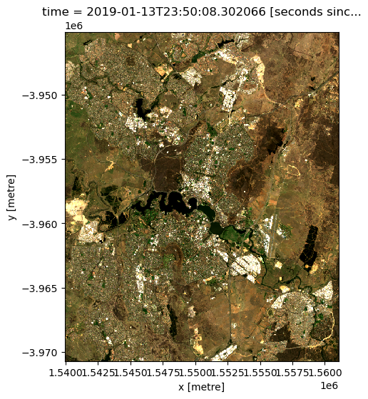
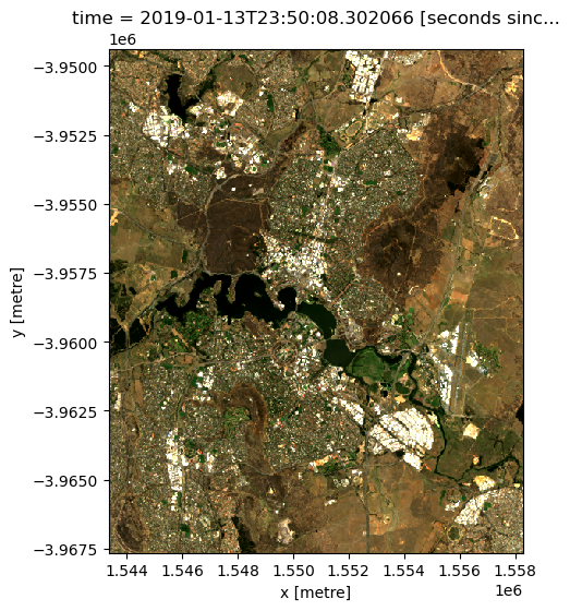
If we plot our satellite data, we can see that it is much higher resolution than our pixelated DEM raster:

rgb(ds)

Reproject datacube data

We can now use the .odc.reproject() method on our existing xarray data to reproject our existing high resolution satellite dataset. We pass raster.odc.geobox to the function to request that the data gets reprojected to match the spatial grid of our low resolution raster.

To control how the data is reprojected, we can specify a custom resampling method that will control how our high resolution pixels will be transformed into lower resolution pixels. In this case, we specify "average", which will set the value of each larger pixel to the average of all smaller pixels that fall within its pixel boundary.

Note: Refer to the odc-geo documentation for a full list of available resampling methods.

# Reproject data
ds_reprojected = ds.odc.reproject(how=raster.odc.geobox, resampling="average")

# Set nodata to `NaN`
ds_reprojected = mask_invalid_data(ds_reprojected)

Now if we plot our reprojected dataset, we can see that our satellite imagery now has a similar resolution to our low resolution raster (e.g. with a pixelated appearance). Note however, that this result will appear smoother than the previous example due to the "average" resampling method used here (compared to "nearest").

rgb(ds_reprojected)

Once again, we can also verify that the two datasets have identical spatial grids:

ds_reprojected.odc.geobox == raster.odc.geobox

True

Loading and reprojecting a raster to match datacube data

Rather than reprojecting satellite data to match the resolution and projection system of our raster, we may instead wish to reproject our raster to match the spatial grid of our satellite data. This can be particularly useful when we have a lower resolution raster file (e.g. like the ~250 m resolution DEM we are using in this example), but we don’t want to lose the better spatial resolution of our satellite data.

Load datacube data

As in the previous example, we can load in satellite data from the datacube at 30 m spatial resolution and Australian Albers (EPSG:3577) coordinate reference system:

# Load data from datacube
ds = dc.load(
    product="ga_ls8c_ard_3",
    measurements=["nbart_red", "nbart_green", "nbart_blue"],
    time=("2019-01-10", "2019-01-15"),
    x=(149.064, 149.205),
    y=(-35.215, -35.365),
    resolution=(-30, 30),
    output_crs="EPSG:3577",
    group_by="solar_day",
)

# Plot 30 m resolution satellite data
rgb(ds)

Load and reproject raster data

We can now use the load_reproject function from dea_tools.datahandling to load and reproject our raster file to match our higher resolution satellite dataset. We pass ds.odc.geobox to the function to request that our raster gets reprojected to match the spatial grid of ds. As in the previous example, we can also specify a custom resampling method which will be used during the reprojection. In this case, we specify 'bilinear', which will produce a smooth output without obvious pixel boundaries.

Note: Refer to the odc-geo documentation for a full list of available resampling methods.

# Load raster and reproject to match satellite dataset
raster_reprojected = load_reproject(
    path=raster_path, how=ds.odc.geobox, resampling="bilinear"
)

# Set nodata to `NaN`
raster_reprojected = mask_invalid_data(raster_reprojected)

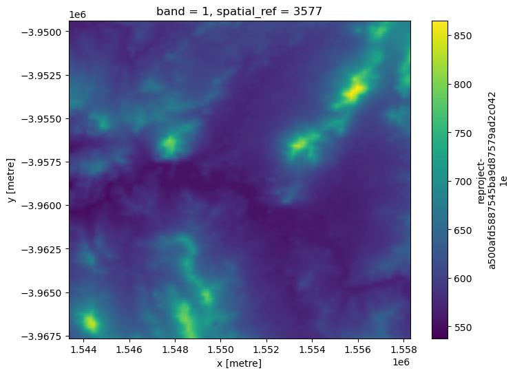
If we plot our resampled raster data, it should now appear less pixelated than the original ~250 m resolution raster.

raster_reprojected.plot(size=6)

/env/lib/python3.10/site-packages/rasterio/warp.py:344: NotGeoreferencedWarning: Dataset has no geotransform, gcps, or rpcs. The identity matrix will be returned.
  _reproject(

<matplotlib.collections.QuadMesh at 0x7f94cc3086a0>

The resampled raster should also match the spatial grid of our higher resolution satellite data:

raster_reprojected.odc.geobox == ds.odc.geobox

True

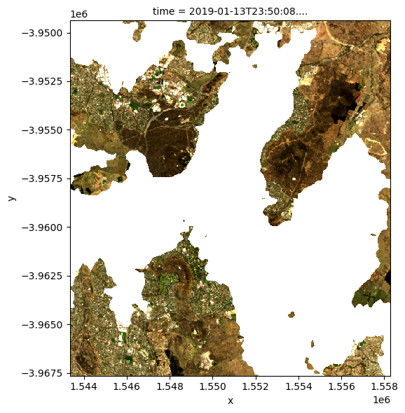
Now both of our datasets share the same spatial grid, we can use our resampled raster to mask our higher resolution satellite dataset as we did in the first section (e.g. mask out all areas lower than 600 m elevation). Compared to the first example, this masked satellite dataset should appear much higher resolution, with far less obvious pixelation:

# Identify hilly areas
is_hilly = raster_reprojected > 600

# Apply mask to set non-hilly areas to `NaN`
ds_masked = ds.where(is_hilly)

# Plot the masked data
rgb(ds_masked, col='time')

---

Additional information

License: The code in this notebook is licensed under the Apache License, Version 2.0. Digital Earth Australia data is licensed under the Creative Commons by Attribution 4.0 license.

Contact: If you need assistance, please post a question on the Open Data Cube Slack channel or on the GIS Stack Exchange using the open-data-cube tag (you can view previously asked questions here). If you would like to report an issue with this notebook, you can file one on GitHub.

Last modified: February 2024

Compatible datacube version:

print(datacube.__version__)

1.8.17

Tags

Tags: NCI compatible, sandbox compatible, landsat 8, rgb, reprojecting data, resampling data, xr_reproject, load_reproject, GeoTIFF, GeoBox, rioxarray.open_rasterio, digital elevation model