Extract and analyse data for multiple polygons

Sign up to the DEA Sandbox to run this notebook interactively from a browser
Compatibility: Notebook currently compatible with both the NCI and DEA Sandbox environments
Products used: ga_ls8c_ard_3

Background

Many users need to run analyses on their own areas of interest. A common use case involves running the same analysis across multiple polygons in a vector file (e.g. ESRI Shapefile or GeoJSON). This notebook will demonstrate how to use a vector file and the Open Data Cube to extract satellite data from Digital Earth Australia corresponding to individual polygon geometries.

Description

If we have a vector file containing multiple polygons, we can use the python package geopandas to open it as a GeoDataFrame. We can then iterate through each geometry and extract satellite data corresponding with the extent of each geometry. Further anlaysis can then be conducted on each resulting xarray.Dataset.

We can retrieve data for each polygon, perform an analysis like calculating NDVI and plot the data.

First we open the vector file as a geopandas.GeoDataFrame
Iterate through each polygon in the GeoDataFrame, and extract satellite data from DEA
Calculate NDVI as an example analysis on one of the extracted satellite timeseries
Plot NDVI for the polygon extent

Getting started

To run this analysis, run all the cells in the notebook, starting with the “Load packages” cell.

Load packages

Note: Please note the use of odc.geo.geom.Geometry: this is important for saving the Coordinate Reference System of the incoming vector in a format that the Digital Earth Australia datacube query can understand.

[1]:

import datacube
import odc.geo.xr
import geopandas as gpd
import matplotlib.pyplot as plt
from odc.geo.geom import Geometry, CRS

import sys

sys.path.insert(1, "../Tools/")
from dea_tools.datahandling import load_ard
from dea_tools.bandindices import calculate_indices
from dea_tools.plotting import rgb
from dea_tools.temporal import time_buffer

Connect to the datacube

Connect to the datacube database to enable loading Digital Earth Australia data.

[2]:

dc = datacube.Datacube(app="Analyse_multiple_polygons")

Analysis parameters

time_of_interest : Enter a time, in units YYYY-MM-DD, around which to load satellite data e.g. '2019-01-01'
time_buff : A buffer of a given duration (e.g. days) around the time_of_interest parameter, e.g. '30 days'
vector_file : A path to a vector file (ESRI Shapefile or GeoJSON)
attribute_col : A column in the vector file used to label the output xarray datasets containing satellite images. Each row of this column should have a unique identifier
products : A list of product names to load from the datacube e.g. ['ga_ls7e_ard_3', 'ga_ls8c_ard_3']
measurements : A list of band names to load from the satellite product e.g. ['nbart_red', 'nbart_green']
resolution : The spatial resolution of the loaded satellite data e.g. for Landsat, this is (-30, 30)
output_crs : The coordinate reference system/map projection to load data into, e.g. 'EPSG:3577' to load data in the Albers Equal Area projection
align : How to align the x, y coordinates respect to each pixel. Landsat Collection 3 should be centre aligned align = (15, 15) if data is loaded in its native UTM zone projection, e.g. 'EPSG:32756'

[3]:

time_of_interest = "2019-02-01"
time_buff = "30 days"

vector_file = "../Supplementary_data/Analyse_multiple_polygons/multiple_polys.shp"
attribute_col = "id"

products = ["ga_ls8c_ard_3"]
measurements = ["nbart_red", "nbart_green", "nbart_blue", "nbart_nir"]
resolution = (-30, 30)
output_crs = "EPSG:3577"
align = (0, 0)

Look at the structure of the vector file

Import the file and take a look at how the file is structured so we understand what we are iterating through. There are two polygons in the file:

[4]:

gdf = gpd.read_file(vector_file)
gdf.head()

[4]:

	id	geometry
0	2	POLYGON ((980959.746 -3560845.144, 983880.024 ...
1	1	POLYGON ((974705.494 -3565359.492, 977625.771 ...

We can then plot the geopandas.GeoDataFrame on an interactive map to make sure it covers the area of interest we are concerned with:

[5]:

gdf.explore(column=attribute_col)

[5]:

Make this Notebook Trusted to load map: File -> Trust Notebook

Create a datacube query object

We then create a dictionary that will contain the parameters that will be used to load data from the DEA data cube:

Note: We do not include the usual x and y spatial query parameters here, as these will be taken directly from each of our vector polygon objects.

[6]:

query = {
    "time": time_buffer(time_of_interest, buffer=time_buff),
    "measurements": measurements,
    "resolution": resolution,
    "output_crs": output_crs,
    "align": align,
}

query

[6]:

{'time': ('2019-01-02', '2019-03-03'),
 'measurements': ['nbart_red', 'nbart_green', 'nbart_blue', 'nbart_nir'],
 'resolution': (-30, 30),
 'output_crs': 'EPSG:3577',
 'align': (0, 0)}

Loading satellite data

Here we will iterate through each row of the geopandas.GeoDataFrame and load satellite data. The results will be appended to a dictionary object which we can later index to analyse each dataset.

[7]:

# Dictionary to save results
results = {}

# Loop through polygons in geodataframe and extract satellite data
for index, row in gdf.iterrows():

    print(f'Feature: {index + 1}/{len(gdf)}')

    # Extract the feature's geometry as a datacube geometry object
    geom = Geometry(geom=row.geometry, crs=gdf.crs)

    # Update the query to include our geopolygon
    query.update({'geopolygon': geom})

    # Load landsat
    ds = load_ard(dc=dc,
                  products=products,
                  # min_gooddata=0.99,  # only take uncloudy scenes
                  ls7_slc_off=False,
                  group_by='solar_day',
                  **query)

    # Mask dataset to set pixels outside the polygon to `NaN`
    ds_masked = ds.odc.mask(poly=geom)

    # Add results to dictionary using the attribute column as an key
    attribute_val = row[attribute_col]
    results[attribute_val] = ds_masked

Feature: 1/2
Finding datasets
    ga_ls8c_ard_3
Applying fmask pixel quality/cloud mask
Loading 3 time steps
Feature: 2/2
Finding datasets
    ga_ls8c_ard_3
Applying fmask pixel quality/cloud mask
Loading 3 time steps

/env/lib/python3.10/site-packages/rasterio/warp.py:344: NotGeoreferencedWarning: Dataset has no geotransform, gcps, or rpcs. The identity matrix will be returned.
  _reproject(

Further analysis

Our results dictionary will contain xarray objects labelled by the unique attribute column values we specified in the Analysis parameters section:

[8]:

results

[8]:

{2: <xarray.Dataset>
 Dimensions:      (time: 3, y: 92, x: 105)
 Coordinates:
   * time         (time) datetime64[ns] 2019-01-17T00:20:13.792499 ... 2019-02...
   * y            (y) float64 -3.561e+06 -3.561e+06 ... -3.564e+06 -3.564e+06
   * x            (x) float64 9.807e+05 9.808e+05 ... 9.838e+05 9.839e+05
     spatial_ref  int32 3577
 Data variables:
     nbart_red    (time, y, x) float32 nan nan nan nan nan ... nan nan nan nan
     nbart_green  (time, y, x) float32 nan nan nan nan nan ... nan nan nan nan
     nbart_blue   (time, y, x) float32 nan nan nan nan nan ... nan nan nan nan
     nbart_nir    (time, y, x) float32 nan nan nan nan nan ... nan nan nan nan
 Attributes:
     crs:           EPSG:3577
     grid_mapping:  spatial_ref,
 1: <xarray.Dataset>
 Dimensions:      (time: 3, y: 92, x: 105)
 Coordinates:
   * time         (time) datetime64[ns] 2019-01-17T00:20:13.792499 ... 2019-02...
   * y            (y) float64 -3.565e+06 -3.565e+06 ... -3.568e+06 -3.568e+06
   * x            (x) float64 9.745e+05 9.745e+05 ... 9.776e+05 9.776e+05
     spatial_ref  int32 3577
 Data variables:
     nbart_red    (time, y, x) float32 nan nan nan nan nan ... nan nan nan nan
     nbart_green  (time, y, x) float32 nan nan nan nan nan ... nan nan nan nan
     nbart_blue   (time, y, x) float32 nan nan nan nan nan ... nan nan nan nan
     nbart_nir    (time, y, x) float32 nan nan nan nan nan ... nan nan nan nan
 Attributes:
     crs:           EPSG:3577
     grid_mapping:  spatial_ref}

Enter one of those values below to index our dictionary and conduct further analysis on the satellite timeseries for that polygon.

[9]:

key = 1

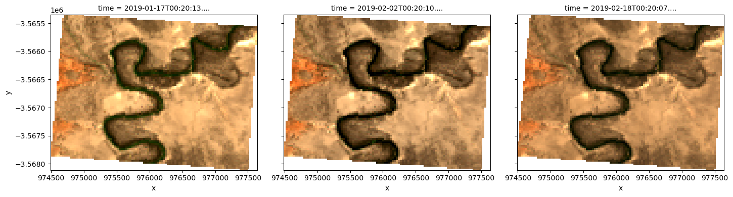
Plot an RGB image

We can now use the dea_plotting.rgb function to plot our loaded data as a three-band RGB plot:

[10]:

rgb(results[key], col="time", size=4)

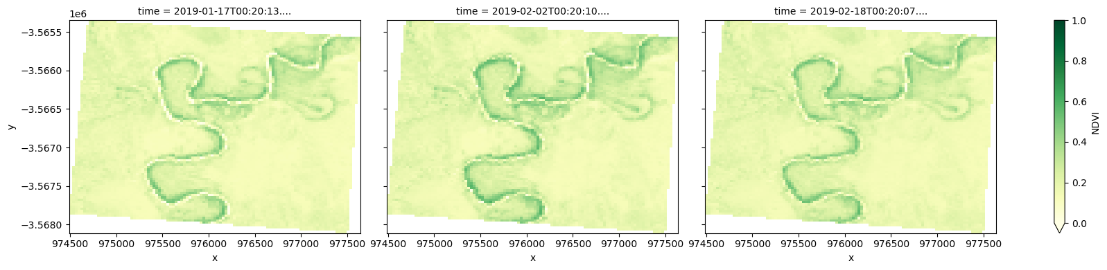
../../../_images/notebooks_How_to_guides_Analyse_multiple_polygons_24_0.png

Calculate NDVI and plot

We can also apply analyses to data loaded for each of our polygons. For example, we can calculate the Normalised Difference Vegetation Index (NDVI) to identify areas of growing vegetation:

[11]:

# Calculate band index
ndvi = calculate_indices(results[key], index="NDVI", collection="ga_ls_3")

# Plot NDVI for each polygon for the time query
ndvi.NDVI.plot(col="time", cmap="YlGn", vmin=0, vmax=1, figsize=(18, 4))
plt.show()

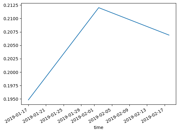
../../../_images/notebooks_How_to_guides_Analyse_multiple_polygons_26_0.png

Plot a NDVI timeseries

Now that we have extracted a masked timeseries for our site of interest, we can summarise each image to produce a timeseries plot of NDVI over time:

[12]:

# Average of NDVI across time
timeseries_df = ndvi.mean(dim=["x", "y"]).drop("spatial_ref").to_dataframe()
timeseries_df.NDVI.plot()

[12]:

<Axes: xlabel='time'>

../../../_images/notebooks_How_to_guides_Analyse_multiple_polygons_28_1.png

We can also export this as a CSV text file:

[13]:

timeseries_df.to_csv(f"timeseries_polygon_{key}.csv")

Additional information

License: The code in this notebook is licensed under the Apache License, Version 2.0. Digital Earth Australia data is licensed under the Creative Commons by Attribution 4.0 license.

Contact: If you need assistance, please post a question on the Open Data Cube Slack channel or on the GIS Stack Exchange using the open-data-cube tag (you can view previously asked questions here). If you would like to report an issue with this notebook, you can file one on GitHub.

Last modified: February 2024

Compatible datacube version:

[14]:

print(datacube.__version__)

1.8.17